Front Matter
Abstract
Problem. Multi-scale systems — ecosystems, institutions, economies, groups of minds, networks of clocks — are assembled from local models that must agree where they overlap. Disagreement comes in kinds. Some can be removed by local adjustment. Some cannot be removed by any local adjustment because it is carried by the topology of the system. Some is generated continuously by local circulation. Version 4.4 of this framework measured disagreement with one scalar (Γ), integrated an excess self-reference over time (K), and asserted cohomological obstructions (H¹) without saying which data carry them [D].
Method. Version 5.0 rebuilds the framework on a single spine: the standard discrete Hodge decomposition of cochains of a cellular sheaf on a finite 2-complex. Every edge datum ω splits orthogonally into a gradient part (removable by re-gauging local states), a harmonic part (a cohomology class, the Draken invariant ϰ) and a curl part (generated by curvature on filled faces). Vertex data x are scored by a resolvent coherence Γ_τ, the normalised cost of the cheapest coherent repair [D].
Results. What is new and what is reused are kept apart throughout. Appendix G classifies every numbered result.
Original to this monograph:
- The anti-totalisation theorem and its admissibility rule. Deleting relations always raises an unanchored coherence measure, so a coherence gain is admissible only on a fixed base, with an excision report attached. The anchored dual, compliance under a declared load, is punished by the same deletion (Theorem 19.2, Prop. 19.6, Cor. 19.5 and 19.7). The mathematics is Loewner monotonicity; the rule is new.
- Principle 2.7: only relational data carry $H^1$; disagreement among local states is an $H^0$ matter. This corrects a confusion that runs through the corpus and v4.4.
- The face-filling reclassification (Prop. 3.7): a measured interior turns a topological obstruction into curvature. Whether a failure reads as “systemic” or “local” is a modelling decision.
- The extension of ϰ to arbitrary relational data (Def. 3.5), and the identification of lifting obstructions with integration obstructions (Prop. 3.11).
- The measurement discipline:
- the resolvent coherence $\Gamma_\tau$ with a declared stiffness and reference (Def. 5.1, Reporting standard 5.7a);
- one dataset scores 0.886 or 0.453 depending only on the declared reference (Ex. 4.1);
- the debiased estimator, the noise floor for ϰ, and the “too good to be true” test (Props. 5.10, 18.1, 18.2);
- “coherence is not soundness” (Prop. 5.8), which withdraws v4.4’s Ψ–Γ conjecture.
- The debt calculus separates gross debt from outstanding balance, and the graded ledger of 28 bridges excludes 7 corpus claims with reasons.
Standard results, reproved in this notation: the Hodge decomposition and its energy identity (Hansen & Ghrist 2019; Lim 2020; Jiang et al. 2011); Tikhonov and GMRF readings of the resolvent; the long exact sequence; Rayleigh monotonicity; and the exact bridges:
- Sagnac synchronisation;
- Berry and Aharonov–Bohm phases as U(1) sheaves;
- CSS and Tanner codes;
- Kuramoto ($r^2=\Gamma_0$, a one-line consequence of the order parameter);
- structural balance;
- Lindeman and Leontief as linear sections.
These bridges are what make the framework’s vocabulary checkable against established science; they are not claimed as discoveries.
All worked examples are recomputed by a published script.
Corrections. Thirteen definitional forks in the corpus are settled (Appendix C). Thirteen arithmetic, logical or bibliographic errors in v4.4 are corrected (Appendix D), including the “Γ < 0 = anti-coherence” reading, which was a normalisation artefact [E].
Scope. This is a theoretical monograph with proofs, computed examples and falsifiable bridges. It is not an empirical validation. Draken is a decoding device that adds explanatory layers to facts, not a prediction machine, and its anti-totalisation principle applies to Draken itself [D].
Keywords: cellular sheaves; Hodge Laplacian; sheaf cohomology; synchronisation; holonomy; quantum codes; Kuramoto; structural balance; coherence measurement; anti-totalisation.
◆ $\min\, S_{\text{sys}}(t)\ \text{ s.t. }\ dH/dt\ge 0$ ◆
How to read this monograph
Epistemic ledger. Every substantive claim paragraph ends with one tag, following the Draken post standard:
| Tag | Meaning |
|---|---|
| [E] | Established: textbook consensus, a proved theorem (proved here or cited), direct measurement |
| [S] | Supported: leading model or majority reading, strong but incomplete evidence |
| [H] | Hypothesis: open, contested, or without decisive evidence |
| [D] | Draken synthesis: a structural claim made by this corpus, submitted for review |
| [M] | Metaphor: a pointer, not a referent; removable without breaking any argument |
A combined tag such as [E/D] means the mathematics is established and the reading of it is Draken synthesis.
Statement types.
- Axioms (A) are modelling commitments.
- Norms (N) are value commitments.
- Theorems and propositions are proved in the text, or cited when standard.
- Hypotheses (H) and predictions (P) are empirical.
Proved results are never cited as evidence for empirical bridges. A bridge earns its status separately (Chapter 10).
What was cut. v4.4’s narrative material is kept in a companion volume, Draken Essays, rather than here. This covers the Levinas reading, the wolf historiography, the cavity resonator, the Marx analysis, nations as minds, and the duty-ethics appendix. It is reinstated only where a chapter below depends on it (Appendix E lists the disposition of every DRK post). Poetic and mythological posts enter only through Knowledge Objects that a chapter uses [D].
Origin of results. Appendix G classifies every numbered result as standard (reproved in this notation, with source), elementary (a short consequence stated for use) or original. The count is 23, 13 and 9 respectively [D].
Running example. The institutional sheaf of Example 4.1 is carried through Chapters 4, 5, 15, 18 and 19. Section 4.9 collects every number computed on it [D].
Reproducibility. Every number in Chapters 4, 5, 13, 15, 16 and 19 is produced by draken_v5_examples.py (Appendix F). Figures 1–6 are its output.
Corpus links. Every DRK mention links to its post at draken.info. DRK-134 is reserved by the corpus index as the companion number to DRK-133 and has no published post, so it is not cited [D].
Part I — Foundations
1 Introduction
1.1 The coherence problem
A complex adaptive system is described by many local models. A trophic ecologist models the wolf–elk interaction, a hydrologist the riverbank, a manager her department, a neuron population its tuning. Each model is valid on its own patch and must agree with its neighbours where the patches overlap. The coherence problem asks three things. Do the local descriptions assemble into one global description? If not, how far are they from doing so? And what kind of failure is it? Sheaf theory is the mathematics of exactly this question: local data, restriction to overlaps, and the obstruction to gluing (Bredon 1997; Curry 2014) [E]. Its cellular, finite-dimensional form makes the question computable with linear algebra (Hansen & Ghrist 2019) [E].
Version 4.4 of this framework (Roininen 2026, the v4.4 monograph, DRK-101–DRK-121) defined a sheaf convergence measure Γ, a narrative self-reference ratio Ψ and a coherence debt K(t). It motivated them with predator–prey ecology. Seventy-two subsequent posts (DRK-123 to DRK-196) extended the formal apparatus in directions v4.4 did not anticipate:
- synchronisation holonomy (The One-Way Gauge, DRK-168; The Dragged Frame, DRK-171);
- the invariant $\varkappa\in H^1$ (The Invariant, DRK-175);
- quantum codes as sheaves (The Warded Class, DRK-190);
- Kuramoto synchrony (The Carrier and the Cargo, DRK-189);
- several new debt integrals.
They also introduced four mutually inconsistent definitions of K, four of Γ and three of Ψ (Appendix C) [E]. Version 5.0 exists to settle these on one mathematical spine [D].
1.2 The core claim
The claim of this monograph has a mathematical half and an empirical half, kept separate throughout.
Mathematical half. Model a multi-scale system as a cellular sheaf $\mathcal F$ on a finite 2-complex $X$, with vertex data $x\in C^0$ (local states) and edge data $\omega\in C^1$ (relational measurements). Then three things hold:
- The incoherence of $x$ is measured by the quadratic form of the sheaf Laplacian.
- The incoherence of $\omega$ splits uniquely and orthogonally into a removable part, a topological part and a curvature part (Theorem 3.1, Proposition 3.2).
- These quantities are computable, carry well-defined invariances, and respond monotonically to adding or deleting relations (Chapter 5).
These are theorems [E].
The central consequence. Every unanchored coherence measure, $\Gamma_\tau$ included, rises when relations are deleted. A system can therefore always look more coherent by ceasing to measure its own disagreements, all the way to Γ = 1 for a system with no relations at all (Theorem 19.2). Coherence gains are admissible only when computed on a fixed base. Measures anchored to a declared load move the other way: deleting relations raises compliance, i.e. the cost of carrying what the system exists to carry (Proposition 19.6). Every diagnostic in this monograph is built so that it cannot be gamed by excision. That design rule is the main contribution, and the rest of the monograph is organised around it [E/D].
Empirical half. The same decomposition, applied to measured data from institutions, ecosystems, nervous systems or markets, separates failures that local repair can fix from failures it cannot. The size and history of the irreducible part predict the magnitude of later corrections (Chapter 22). This is a research programme, not a result [H].
1.3 The decoding stance
Draken is a device for adding explanatory layers to facts. It is not a machine for predicting them. A Draken reading of a case is useful when it identifies:
- which disagreements are local (gradient);
- which are structural (harmonic);
- which are being generated by circulation (curl).
It is useless when it is used to totalise: to declare one global section true and the rest noise. The framework’s own anti-totalisation result (Chapter 19) applies to Draken: a version of this framework that raised its coherence by deleting its inconvenient posts would be committing the error it diagnoses [D].
1.4 Relationship to existing frameworks
The Draken apparatus is assembled almost entirely from established parts:
- Cellular sheaves and their Laplacians come from Curry (2014) and Hansen & Ghrist (2019), and opinion dynamics on discourse sheaves from Hansen & Ghrist (2021) [E].
- The combinatorial Hodge decomposition of edge flows is standard (Lim 2020). Its use for ranking and inconsistency analysis is HodgeRank (Jiang, Lim, Yao & Ye 2011) [E].
- Connection Laplacians and their frustration bounds come from Singer & Wu (2012) and Bandeira, Singer & Spielman (2013) [E].
- Learned sheaves on graphs come from Bodnar et al. (2022) and Barbero et al. (2022) [E].
- Graph signal processing supplies the resolvent (Tikhonov) smoother used for Γ_τ (Shuman et al. 2013) [E].
- Active inference supplies the variational reading of diffusion (Friston 2010) [E].
- Sheaves as the data structure for fusing heterogeneous sensors are due to Robinson (2017). Estimation from relative measurements, with error governed by effective resistance, is due to Barooah & Hespanha (2008) [E].
What is original to Draken:
- the multi-scale ontology (Section 2.6);
- the system of diagnostic measures and their reporting discipline (Chapters 5–9);
- the debt calculus (Chapter 7);
- the anti-totalisation theorem and its admissibility rule (Chapter 19);
- the claim that these one-and-the-same objects recur at scales from clocks to institutions (Part III).
Of these, the last is the claim most in need of empirical defence [D].
1.5 Scope and limitations
The monograph proves what it can prove and labels the rest.
- It does not claim that social or ecological systems are sheaves. It claims that sheaves are the right bookkeeping for local-to-global consistency, and that the bookkeeping exposes distinctions that scalar indices hide [D].
- Every application requires a declared complex, declared stalks, declared restriction maps and a declared measurement protocol. Without these, no Draken number has meaning (Axiom A2) [D].
- Worked examples on synthetic data are proofs of computability, not validations [E].
1.6 Source hierarchy
Claims are weighted in the following order:
- Proved results and peer-reviewed literature, cited by author and year.
- Preprints, marked [S] at most.
- DRK posts, cited as corpus synthesis [D] and never as external evidence.
- Etymological and mythological readings, marked [M] and never load-bearing.
A [D] claim never cites an external source as if that source had made it [D].
1.7 The predator, briefly
The framework began with an ecological observation. Removing an apex predator from Yellowstone was followed by changes in elk behaviour, browse pressure and riparian vegetation (Ripple & Beschta 2004). The strength and attribution of that cascade remain debated (Ripple et al. 2025; MacNulty et al. 2025) [S].
The structural reading that survives into v5.0 is narrower. An agent that enforces consistency between scales acts like a restriction map that is actually checked. Removing it does not create disagreement directly. It removes the place where disagreement was being measured and paid for (Chapter 19) [D]. The broader predator material of v4.4 is kept in the companion volume [D].
2 Axioms and the formal setting
2.1 Axioms and norms
The framework rests on five modelling axioms and two norms. The axioms say what a Draken model is. The norms say what a Draken intervention may do. Neither kind is an empirical claim [D].
Axiom A0 (Finiteness). Every model is a finite cell complex with finite-dimensional stalks. Real numbers enter only as the field of coefficients for measurement; every computation is a finite linear-algebra computation. This adopts the operational core of The Finite Sheaf (DRK-141) without its further claims about quantum probability (Chapter 14) [D].
Axiom A1 (Sheaf modelling). A system is modelled by:
- a regular 2-complex $X$, whose vertices are local models, whose edges are declared overlaps or relations, and whose faces are declared closed loops of relations;
- a cellular sheaf $\mathcal F$ on $X$ (Definition 2.2);
- data: vertex states $x\in C^0(X;\mathcal F)$ and/or relational measurements $\omega\in C^1(X;\mathcal F)$ [D].
Axiom A2 (Declared geometry). Every stalk carries a declared inner product. Every comparison between systems, or across time, uses the same complex, stalks, inner products, restriction maps and stiffness τ (Chapter 5). A number reported without its declared geometry is not a Draken measurement [D].
Axiom A3 (Base-fixity). Coherence gains are admissible only when computed on a fixed base. A change of base (deleting cells, zeroing stalks) is reported separately as an excision, with its cost (Definition 19.3) [D].
Axiom A4 (Coefficient declaration). Measurements are taken over $\mathbb R$ (or $\mathbb C$ for phase data). Obstructions with torsion, such as orientation and sign consistency, are invisible over a field of characteristic zero. They require $\mathbb Z$ or $\mathbb F_2$ coefficients, and these must be declared when relevant (Remark 3.8) [E/D].
Norm N1 (Optimization axiom). Interventions are evaluated by $$\Diamond\quad \min_{\pi}\ S_{\text{sys}}(t)\quad\text{subject to}\quad \frac{dH}{dt}\ \ge\ 0\quad\Diamond$$ where $S_{\text{sys}}$ is the disorder of the system (thermodynamic or functional entropy, declared per application) and $H$ is its structural diversity (Shannon entropy of the distribution of distinguishable components, declared per application). In words: reduce disorder without simplifying away complexity. Its verbal form is the approved KO from Drakens Ordlista (DRK-117) [D].
Norm N2 (Care). An agent’s own contribution to the variety of the systems it is coupled to is held at zero: $\dot{\mathcal V}_{\text{exo}}=0$ (KO from The Bridge and the Burn, DRK-162). Violations in the destructive direction accrue trophic debt Θ (Chapter 7) [D].
The norms constrain interventions. The anti-totalisation theorem (Chapter 19) shows why N1 cannot be met by excision, and Chapter 9 shows why N2 protects the invariant [D].
2.2 Cell complexes
Definition 2.1 (Regular 2-complex). A finite regular CW complex $X$ of dimension at most 2 has three kinds of cells:
- vertices $V$, edges $E$ and faces $F$;
- a face relation $\sigma\trianglelefteq\tau$ (“σ is a face of τ”);
- incidence numbers $[\sigma:\tau]\in\{-1,0,+1\}$ for cells of adjacent dimension.
The incidence numbers satisfy $$\sum_{\sigma}[\rho:\sigma][\sigma:\tau]=0\qquad\text{whenever }\dim\rho=\dim\tau-2.$$ Graphs are the case $F=\emptyset$. For an oriented edge $e=(u\to v)$, take $[u:e]=-1$ and $[v:e]=+1$ [E].
The identity above encodes “the boundary of a boundary is zero”. It is the only combinatorial fact the theory needs (Curry 2014) [E].
2.3 Cellular sheaves
Definition 2.2 (Cellular sheaf). A cellular sheaf $\mathcal F$ on $X$ consists of:
- a finite-dimensional real (or complex) inner-product space $\mathcal F(\sigma)$, the stalk, on each cell;
- a linear restriction map $\mathcal F_{\sigma\trianglelefteq\tau}:\mathcal F(\sigma)\to\mathcal F(\tau)$ for each face relation;
subject to identity and composition: $$\mathcal F_{\sigma\trianglelefteq\sigma}=\mathrm{id},\qquad \mathcal F_{\rho\trianglelefteq\tau}=\mathcal F_{\sigma\trianglelefteq\tau}\,\mathcal F_{\rho\trianglelefteq\sigma}.$$ (Curry 2014; Hansen & Ghrist 2019) [E].
The corpus writes restriction maps as $\rho$. That shorthand is the approved KO ρ (Drakens Ordlista, DRK-117) and is retained: $\rho_{\sigma\tau}:=\mathcal F_{\sigma\trianglelefteq\tau}$. To avoid the collisions found in the corpus, the symbol $\rho$ is reserved for restriction maps in this monograph; density is written $\varrho$ and a density matrix $\hat\rho$ (Appendix A) [D].
Direction. Cellular sheaves map from lower-dimensional cells to the cells that contain them. A vertex’s state is pushed onto each edge it meets, where it is compared with the neighbour’s. This is the opposite variance to the textbook “restrict from large open sets to small ones”. The two pictures agree once $X$ carries the Alexandrov topology, in which the smallest open set containing a cell is its open star (Curry 2014) [E].
Proposition 2.3 (Stalks of a cellular sheaf). In the Alexandrov topology on the face poset of $X$, the stalk of $\mathcal F$ at a cell $\sigma$, $$\mathcal F_\sigma=\varinjlim_{U\ni\sigma}\mathcal F(U),$$ equals $\mathcal F(\sigma)$. The approved KO stalk (The Stal King, DRK-192) therefore coincides, for cellular sheaves, with the stalk space on the cell [E].
Proof. There are two steps.
- The colimit. Order the open neighbourhoods of σ by reverse inclusion. Every one of them contains the open star $\mathrm{st}(\sigma)$, which is itself open, so $\mathrm{st}(\sigma)$ is the terminal object of this directed system. A colimit over a diagram with a terminal object is the value at that object: $\mathcal F_\sigma=\mathcal F(\mathrm{st}(\sigma))$.
- The value on the star. For a cellular sheaf, the sections over an open set $U$ are the limit of $\mathcal F$ over the cells of $U$. In $\mathrm{st}(\sigma)$ the cell σ is a face of every other cell, so σ is initial in that diagram, and a limit over a diagram with an initial object is the value at that object: $\mathcal F(\mathrm{st}(\sigma))=\mathcal F(\sigma)$. ∎
2.4 Cochains and the coboundary
Definition 2.4. The $k$-cochains are $C^k=C^k(X;\mathcal F)=\bigoplus_{\dim\sigma=k}\mathcal F(\sigma)$, with the orthogonal direct-sum inner product. The coboundary $\delta^k:C^k\to C^{k+1}$ is $$(\delta^k x)_\tau=\sum_{\sigma\trianglelefteq\tau,\ \dim\sigma=k}[\sigma:\tau]\,\mathcal F_{\sigma\trianglelefteq\tau}\,x_\sigma .$$ For an edge $e=(u\to v)$ this reads $$(\delta^0x)_e=\mathcal F_{v\trianglelefteq e}x_v-\mathcal F_{u\trianglelefteq e}x_u,$$ which is the disagreement of the two endpoint states on the shared edge stalk [E].
Lemma 2.5 ($\delta\delta=0$). $\delta^{1}\delta^{0}=0$.
Proof. For a face τ and a vertex ρ ≤ τ, $$(\delta^1\delta^0x)_\tau=\sum_{\rho}\Big(\sum_{\sigma}[\rho:\sigma][\sigma:\tau]\Big)\mathcal F_{\rho\trianglelefteq\tau}\,x_\rho .$$ This uses composition, $\mathcal F_{\sigma\trianglelefteq\tau}\mathcal F_{\rho\trianglelefteq\sigma}=\mathcal F_{\rho\trianglelefteq\tau}$. The inner sum vanishes by Definition 2.1. ∎ [E]
The lemma is the formal content of the slogan “local consistency is necessary for global consistency”. Every gradient datum is automatically curvature-free [E/D].
Remark 2.5a (Orientation and reciprocity). A 1-cochain is defined relative to the orientation of each edge. Reversing the orientation of $e$ negates $\omega_e$, so relational data are antisymmetric by construction: $\omega_{v\to u}=-\omega_{u\to v}$. Wrestling with God (DRK-142) reads Newton’s third law, $\mathbf F_{B\to A}=-\mathbf F_{A\to B}$, as the condition that force in grappling cannot be unilateral. In v5.0 that reading is the orientation axiom of $C^1$: an exchange is one cochain value seen from its two ends (§16.1) [E/D].
2.5 Cohomology, global sections, obstruction
Definition 2.6. The cohomology groups are $$H^0=\ker\delta^0,\qquad H^1=\ker\delta^1/\operatorname{im}\delta^0,$$ and the Betti numbers are $b_k=\dim H^k$.
Elements of $H^0$ are the global sections: vertex states that agree on every edge. This is the approved KO global section (The Operational Question in Positive Alignment, DRK-145). A nonzero class in $H^1$ is the approved KO cohomological obstruction (Drakens Ordlista, DRK-117) [E/D].
What $H^1$ obstructs needs to be stated precisely, because v4.4 and several posts state it loosely.
Principle 2.7 (Who carries $H^1$). Vertex data alone never exhibit an $H^1$ obstruction. For any $x\in C^0$, the disagreement $\delta^0x$ lies in $\operatorname{im}\delta^0$ and has zero class in $H^1$. Disagreement among vertex states is an $H^0$ phenomenon: it measures how far $x$ is from $\ker\delta^0$.
An $H^1$ obstruction appears only when the data include relational measurements $\omega\in C^1$ that are not computed from vertex states. Examples:
- clock offsets measured on links;
- pairwise comparisons;
- exchange rates;
- parallel transport of frames;
- the signs of alliances;
- syndromes of a code.
Each of these poses the integration problem: find $x$ with $\delta^0x=\omega$. The problem is solvable exactly when $\omega\in\operatorname{im}\delta^0$. For closed ω ($\delta^1\omega=0$) the obstruction to solving it is the class $[\omega]\in H^1$ [E].
Every $H^1$ claim in this monograph therefore names its relational datum. Claims in the corpus that attribute $H^1$ to disagreement among vertex states are restated as $H^0$ claims (Appendix C, fork F6) [D].
2.6 The multi-scale template
The Draken ontology is a modelling template, not a metaphysics. Following v4.4 (authoritative for layer definitions), it decomposes systems into eighteen layers in five bands. The number 18 is a resolution choice; the mathematics applies to any finite decomposition with declared inter-layer restriction maps [D].
| Band | Layer | Name | Emergent agent | Typical data | Dominant dynamics |
|---|---|---|---|---|---|
| Substrate | L01 | Quantum / field substrate | Physical patterns | Field amplitudes, symmetry parameters | Symmetry-breaking, pattern formation |
| L02 | Chemical / dissipative | Chemical agents | Concentration fields, reaction rates | Dissipative structure formation | |
| L03 | Molecular assembly | Biological polymers | Sequence data, folding states | Self-assembly, molecular recognition | |
| L04 | Bioelectric / tissue patterning | Cellular ensembles | Membrane potentials, morphogen gradients | Bioelectric signalling, development | |
| Organismal | L05 | Neural integration | Neural agents | Firing rates, synaptic weights | Predictive coding, Hebbian learning |
| L06 | Embodied cognition | Sensorimotor agents | Proprioceptive states, motor plans | Enactivism, allostasis | |
| L07 | Narrative self | Autobiographical agents | Belief states, self-models | Active inference, identity maintenance | |
| L08 | Dyadic bonds | Relational agents | Attachment states, trust levels | Reciprocity, pair-bonding | |
| Social | L09 | Group cognition | Collective agents | Shared beliefs, norms | Coalitional games, reputation |
| L10 | Institutional coordination | Institutional agents | Rules, procedures, roles | Isomorphism, principal–agent | |
| L11 | Economic exchange | Market agents | Prices, contracts, flows | Equilibrium, input–output | |
| L12 | Collective narratives | Narrative agents | Media content, public opinion | Memetic dynamics, opinion formation | |
| Structural | L13 | Political structure | Governance agents | Constitutions, laws, policies | Legitimacy, power transitions |
| L14 | Economic topology | Macroeconomic agents | GDP, trade flows, capital stocks | Growth, business cycles | |
| L15 | Cultural field | Cultural agents | Values, aesthetics, ideologies | Cultural evolution, field dynamics | |
| L16 | Institutional morphology | Meta-institutional agents | Constitutional orders, treaties | Regime transitions, path dependence | |
| Planetary | L17 | Civilizational memory | Civilizational agents | Archives, traditions, canons | Long-duration processes |
| L18 | Planetary cognition | Planetary agents | Climate, biosphere state | Earth-system dynamics |
Status of the template. No worked example in this monograph instantiates the eighteen layers. Examples 4.1–4.8 use small, declared complexes, and no inter-layer restriction map is estimated here. The table is the declared cover the corpus uses for its readings. It carries no evidential weight, and nothing proved in Parts I–V depends on it [D].
Layer complexes. A layer complex places one or more vertices per layer, edges between layers that constrain each other, and faces on loops of constraints that are jointly measured. Inter-layer restriction maps are estimated, not assumed. The linear estimator from v4.4 remains the default: $$\rho^\ast_{ij}=\arg\min_{R}\sum_t\big\|R\,x_i(t)-x_j(t)\big\|^2,$$ with residuals reported. Non-linear constraints are handled by local linearisation (Jacobians at the operating point), by kernel lifting, or by learned maps (Bodnar et al. 2022). Spectral statements then hold only locally and must be reported with their validity region [E/D].
Emergence. At each scale, interacting agents give rise to emergent agents one scale up (Prigogine & Stengers 1984; Kauffman 1993) [S]. In sheaf terms, an emergent agent is a vertex at layer $n+1$ whose stalk is the image of a restriction from a subcomplex at layer $n$. It persists when that restriction is stable under the dynamics of Chapter 15 [D].
3 The Hodge Spine
This chapter is the mathematical centre of v5.0. Everything in Parts II–V is a reading of, a measure on, or a dynamics for the decomposition proved here [D].
3.1 Adjoints and Hodge Laplacians
With the declared inner products (Axiom A2), each coboundary has an adjoint $\delta^{k*}$. For real stalks with orthonormal bases, $\delta^{k*}=\delta^{k\top}$.
Definition 3.0. The Hodge Laplacians of $\mathcal F$ are $$\Delta^0=\delta^{0*}\delta^0,\qquad \Delta^1=\delta^0\delta^{0*}+\delta^{1*}\delta^1,\qquad \Delta^2=\delta^1\delta^{1*}.$$ $\Delta^0$ is the sheaf Laplacian $L_{\mathcal F}$. This is the approved KO from The Operational Question in Positive Alignment (DRK-145), there written $\Delta_{\mathcal F}=\delta^\top\delta$ [E].
Its quadratic form is the total disagreement energy (Hansen & Ghrist 2019) [E]: $$E(x):=\langle x,L_{\mathcal F}x\rangle=\|\delta^0x\|^2=\sum_{e=(u\to v)}\big\|\rho_{ve}x_v-\rho_{ue}x_u\big\|^2 .$$
3.2 The decomposition
Theorem 3.1 (Hodge decomposition). For $k=0,1,2$ there is an orthogonal decomposition $$C^k=\operatorname{im}\delta^{k-1}\ \oplus\ \ker\Delta^k\ \oplus\ \operatorname{im}\delta^{k*},$$ with $\ker\Delta^k=\ker\delta^k\cap\ker\delta^{k-1*}$ and $\ker\Delta^k\cong H^k$. (Terms with out-of-range indices are zero.)
Proof.
- Kernel of $\Delta^k$. For any $c$, $$\langle\Delta^kc,c\rangle=\|\delta^kc\|^2+\|\delta^{k-1*}c\|^2,$$ so $\Delta^kc=0$ if and only if $\delta^kc=0$ and $\delta^{k-1*}c=0$.
- Orthogonality of the outer summands. By Lemma 2.5, $$\langle\delta^{k-1}a,\ \delta^{k*}b\rangle=\langle\delta^k\delta^{k-1}a,\ b\rangle=0 .$$
- The complement. In finite dimensions, $(\operatorname{im}\delta^{k-1})^\perp=\ker\delta^{k-1*}$ and $(\operatorname{im}\delta^{k*})^\perp=\ker\delta^k$. The orthogonal complement of $\operatorname{im}\delta^{k-1}\oplus\operatorname{im}\delta^{k*}$ is therefore $\ker\delta^{k-1*}\cap\ker\delta^k=\ker\Delta^k$.
- The isomorphism. Since $\operatorname{im}\delta^{k-1}\subseteq\ker\delta^k$, we have $\ker\delta^k=\operatorname{im}\delta^{k-1}\oplus\ker\Delta^k$. Hence $H^k=\ker\delta^k/\operatorname{im}\delta^{k-1}\cong\ker\Delta^k$. ∎
This is the finite-dimensional Hodge theorem for cochain complexes. For cellular sheaves it is in Hansen & Ghrist (2019); for graphs and edge flows, in Lim (2020) and Jiang et al. (2011) [E].
For edge data $\omega\in C^1$, write $\Pi_{\text{grad}},\Pi_{\text{harm}},\Pi_{\text{curl}}$ for the three orthogonal projectors. Then $$\boxed{\ \omega\;=\;\underbrace{\delta^0x^\star}_{\text{gradient}}\;+\;\underbrace{h}_{\text{harmonic}}\;+\;\underbrace{\delta^{1*}y}_{\text{curl}}\ },\qquad x^\star=(\delta^0)^{+}\omega,$$ where $^+$ is the Moore–Penrose pseudoinverse [E].
3.3 Energies and the integration problem
Proposition 3.2 (Energy identity; least squares). For $\omega\in C^1$:
$\|\omega\|^2=E_{\text{grad}}+E_{\text{harm}}+E_{\text{curl}}$, with $E_\bullet=\|\Pi_\bullet\omega\|^2$.
$\displaystyle\min_{x\in C^0}\|\omega-\delta^0x\|^2=E_{\text{harm}}+E_{\text{curl}}$.
The minimisers are exactly $x^\star+H^0$.
Proof. (i) is Pythagoras for orthogonal summands. For (ii), $\delta^0x$ ranges over $\operatorname{im}\delta^0$, so the minimum is the squared distance from ω to that subspace, which is the norm of its orthogonal remainder. For (iii), $\delta^0x=\Pi_{\text{grad}}\omega$ holds if and only if $x-x^\star\in\ker\delta^0=H^0$. ∎ [E]
Definition 3.2a (Obstruction energy). $E_{\text{obs}}(\omega):=E_{\text{harm}}+E_{\text{curl}}$ is the part of the relational data that no assignment of local states can reproduce. The integrability share is $$\Gamma^1(\omega):=E_{\text{grad}}/\|\omega\|^2\in[0,1],$$ and its complement $1-\Gamma^1$ is the obstruction share [D].
3.4 Gauge invariance
A gauge transformation re-expresses every local state by an offset: $x\mapsto x+g$ for $g\in C^0$. Relational data change accordingly, $\omega\mapsto\omega+\delta^0g$. Re-zeroing every clock, re-basing every price, or re-anchoring every local convention are gauge transformations [E].
Proposition 3.3. $\Pi_{\text{harm}}$, $\Pi_{\text{curl}}$, the curvature $\delta^1\omega$, $E_{\text{harm}}$ and $E_{\text{curl}}$ are gauge invariant.
Proof. $\delta^0g\in\operatorname{im}\delta^0$ is annihilated by $\Pi_{\text{harm}}$ and $\Pi_{\text{curl}}$, and by $\delta^1$ (Lemma 2.5). ∎ [E]
Reading: no choice of local conventions can create or destroy the topological or curvature part of a disagreement. Only the gradient part is convention-dependent [E/D].
3.5 Curvature
Proposition 3.4 (Curvature determines the curl). Let $\mathcal R:=\delta^1\omega\in C^2$ be the curvature of ω. Then $$\Pi_{\text{curl}}\,\omega=\delta^{1*}\,(\delta^1\delta^{1*})^{+}\,\mathcal R,\qquad E_{\text{curl}}=\big\langle \mathcal R,\ (\Delta^2)^{+}\mathcal R\big\rangle .$$ Moreover, ω is closed ($\mathcal R=0$) if and only if its curl part vanishes.
Proof. $\delta^1$ annihilates the gradient part (Lemma 2.5) and the harmonic part (Theorem 3.1), so $\mathcal R=\delta^1\delta^{1*}y$. Choosing $y\in\operatorname{im}\delta^1$ (always possible) gives $y=(\Delta^2)^{+}\mathcal R$. Then $$E_{\text{curl}}=\langle\delta^{1*}y,\delta^{1*}y\rangle=\langle y,\Delta^2y\rangle=\langle\mathcal R,(\Delta^2)^+\mathcal R\rangle .$$ If $\mathcal R=0$ then $y=0$. Conversely, $\delta^1$ is injective on $\operatorname{im}\delta^{1*}$, so a nonzero curl part has nonzero curvature. ∎ [E]
The formula is verified numerically in Example 4.4 ($E_{\text{curl}}$ by projection and by curvature agree to $10^{-6}$) [E].
3.6 The invariant ϰ
Definition 3.5 (Draken invariant). For $\omega\in C^1$, $$\varkappa(\omega):=[\,\Pi_{\text{harm}}\,\omega\,]\in H^1(X;\mathcal F),\qquad b_1(\mathcal F)=\dim H^1 .$$
When ω is closed, $\varkappa(\omega)=[\omega]$. This is the approved KO definition $\varkappa:=[\omega]\in H^1(X,\mathcal F)$ of The Invariant (DRK-175). Definition 3.5 extends it to arbitrary relational data, which in applications are never exactly closed [E/D].
Proof of the reduction. A closed ω has no curl part (Proposition 3.4), so $\omega=\delta^0x^\star+h$ and $[\omega]=[h]$. ∎ [E]
This extension removes the inconsistency between The Invariant (DRK-175) and Ouroboros Debt (DRK-176):
- DRK-175 requires $[\omega]$ and therefore $\delta\omega=0$.
- DRK-176 accrues debt from $\|d\omega\|\neq 0$.
In v5.0 both hold for the same ω. The harmonic part carries ϰ; the curvature carries the curl energy, whose time integral is the curvature load $C(t)$ of Chapter 7 [D].
Proposition 3.6 (Periods). Let $\mathcal F$ be a constant sheaf $\mathbb R$ on $X$. The period of a 1-cochain on an oriented cycle γ is $\langle\omega,\gamma\rangle=\sum_{e\in\gamma}\pm\omega_e$.
Periods of $h=\Pi_{\text{harm}}\omega$ depend only on the homology class of γ. They determine $\varkappa(\omega)$, since $H^1(X;\mathbb R)\cong\operatorname{Hom}(H_1(X),\mathbb R)$.
Periods of ω itself satisfy a discrete Stokes formula: if $\gamma-\gamma'=\partial c$ for a 2-chain $c$, then $$\langle\omega,\gamma\rangle-\langle\omega,\gamma'\rangle=\langle\mathcal R,c\rangle .$$
Proof. (i) Harmonic cochains are closed, so their periods vanish on boundaries. The isomorphism is the universal coefficient theorem over a field (Hatcher 2002). (ii) $\langle\omega,\partial c\rangle=\langle\delta^1\omega,c\rangle$ by the definition of $\delta^1$ as the transpose of $\partial$. ∎ [E]
Reading: when relational data have curvature, “the discrepancy around a loop” is not well defined, because it depends on which loop represents the hole. ϰ assigns each hole a single period, the least-squares reconciliation of all representatives. In Example 4.4 the two loops around the open hole have periods 0.03 and 0.06; ϰ assigns 0.04 [E/D].
3.7 What counts as a hole is a modelling decision
Proposition 3.7 (Face filling reclassifies obstruction). Let $X'=X\cup\{\tau\}$, adding one face whose boundary is a cycle in $X$, and let $\mathcal F'$ extend $\mathcal F$. For every $\omega\in C^1$ (unchanged by the filling):
$E'_{\text{grad}}=E_{\text{grad}}$;
$E'_{\text{curl}}\ge E_{\text{curl}}$ and $E'_{\text{harm}}\le E_{\text{harm}}$, with $E'_{\text{harm}}+E'_{\text{curl}}=E_{\text{harm}}+E_{\text{curl}}$;
$b_1'=b_1-(\operatorname{rank}\delta'^1-\operatorname{rank}\delta^1)$. For the constant scalar sheaf and a cycle that is not already a boundary, $b_1'=b_1-1$.
Proof. $C^0$, $C^1$ and $\delta^0$ are unchanged, so the gradient projection is unchanged. $\operatorname{im}\delta'^{1*}\supseteq\operatorname{im}\delta^{1*}$, and orthogonal projection onto a larger subspace has a larger norm. The sum is fixed by (i) and Proposition 3.2. Part (iii) is rank–nullity. ∎ [E]
The proposition says that whether an irreducible disagreement is topological (harmonic) or local circulation (curl) depends on whether the region it encircles is part of the declared base. An unmeasured interior is a hole. A measured interior is a source of curvature. This is why Axiom A2 requires the faces to be declared, and it resolves an ambiguity in the corpus’s physics posts (Chapter 10) [D].
3.8 Coefficients and torsion
Remark 3.8. Over a field of characteristic zero, torsion in integral homology disappears. The Klein bottle $K$ has $H_1(K;\mathbb Z)\cong\mathbb Z\oplus\mathbb Z/2$, but $H_1(K;\mathbb R)\cong\mathbb R$; the $\mathbb Z/2$ class, which is the failure of orientability, is invisible to real-valued measurement (Hatcher 2002) [E].
The Bottle Has No Outside (DRK-187) reads non-orientability as the absence of a view from outside. The precise residue of that reading is Axiom A4: obstructions of sign or orientation type must be measured with $O(1)$-valued restriction maps (signed sheaves, Section 4.7) or over $\mathbb F_2$ (codes, Chapter 12) [D].
3.9 Two faces of $H^1$
The same group plays two roles, and it is reached by two roads (integration, here, and lifting, §3.10):
- In an integration problem (clocks, prices, comparisons), a nonzero class is what cannot be made consistent. It is an obstruction.
- In a code (Chapter 12), a nonzero class is what local errors cannot change without crossing the code distance. It is protected information: the number of logical qubits of a CSS code is $\dim H_1$ (Calderbank & Shor 1996; Kitaev 2003).
Draken’s normative stance follows the second face as well as the first. A healthy system keeps a bounded, named, nonzero ϰ: irreducible difference that is held rather than erased (The Invariant, DRK-175, §5) [E/D].
3.10 Extensions: the second road to $H^1$
Principle 2.7 reaches $H^1$ through the integration problem: can relational data be integrated into local states? The corpus reaches the same group by a second road, the lifting problem of The Cloven Section (DRK-174): can a visible quotient be lifted back into the whole it was cut from? This section shows that the two roads meet. Every lifting obstruction is the integration obstruction of a derived relational datum, and the Hodge spine applies to it unchanged [D].
Definition 3.9 (Short exact sequence of sheaves). A sequence of cellular sheaves on $X$, $$0\longrightarrow\mathcal K\xrightarrow{\ i\ }\mathcal E\xrightarrow{\ p\ }\mathcal Q\longrightarrow0,$$ is short exact if two conditions hold:
- on every cell σ, $0\to\mathcal K(\sigma)\to\mathcal E(\sigma)\to\mathcal Q(\sigma)\to0$ is exact;
- $i$ and $p$ commute with all restriction maps.
DRK-174 uses three readings of the terms:
- $p$ is the cut, clēofan;
- $\mathcal K$ is what the cut forgets;
- a section $s$ with $p\circ s=\mathrm{id}$ is the re-adhering, clifian [E/D].
Theorem 3.10 (Long exact sequence). A short exact sequence of cellular sheaves induces the exact sequence $$0\to H^0(\mathcal K)\to H^0(\mathcal E)\to H^0(\mathcal Q)\xrightarrow{\ \partial\ }H^1(\mathcal K)\to H^1(\mathcal E)\to H^1(\mathcal Q)\to\cdots .$$ The connecting map is computed as follows. Lift $q\in H^0(\mathcal Q)$ stalkwise to some $e\in C^0(\mathcal E)$. Then $\delta_{\mathcal E}e$ lies in $i\,C^1(\mathcal K)$, and $\partial q=[\,i^{-1}\delta_{\mathcal E}e\,]$.
Proof. Stalkwise exactness and compatibility with restriction maps give a short exact sequence of cochain complexes. The snake lemma then yields the long exact sequence and the stated formula (Weibel 1994, Thm. 1.3.1). For well-definedness: $p\,\delta_{\mathcal E}e=\delta_{\mathcal Q}q=0$, so $\delta_{\mathcal E}e\in\ker p=\operatorname{im}i$ on every edge. ∎ [E]
Proposition 3.11 (Lifting is integration). Let $q\in H^0(\mathcal Q)$ and choose any stalkwise lift $e$. Put $\omega_q:=i^{-1}\delta_{\mathcal E}e\in C^1(\mathcal K)$. Then:
$\omega_q$ is closed: $\delta^1_{\mathcal K}\omega_q=0$. Its curl part vanishes.
The global lifts of $q$ are exactly $e-i\,k$ with $\delta^0_{\mathcal K}k=\omega_q$. Hence $q$ lifts if and only if $\varkappa(\omega_q)=\partial q=0$.
A different stalkwise lift changes $\omega_q$ by a gradient. So $\varkappa(\omega_q)$ and $E_{\text{harm}}(\omega_q)$ depend on $q$ alone.
If each $i_\sigma$ is an isometry, the least disagreement achievable by any lift is $$\min_{\tilde e:\ p\tilde e=q}\|\delta_{\mathcal E}\tilde e\|^2=E_{\text{harm}}(\omega_q).$$
Proof.
$\delta^1_{\mathcal E}\delta^0_{\mathcal E}e=0$ by Lemma 2.5, and $i$ is injective.
$p(e-ik)=q$. Moreover $\delta_{\mathcal E}(e-ik)=i(\omega_q-\delta_{\mathcal K}k)$, which vanishes if and only if $\delta_{\mathcal K}k=\omega_q$. Every lift of $q$ has this form, because two lifts differ by an element of $\ker p=\operatorname{im}i$. The class statement follows from Definition 3.5 and Theorem 3.10.
Two lifts differ by $ik'$, which changes $\omega_q$ by $\delta_{\mathcal K}k'$. Apply Proposition 3.3.
By (ii) and isometry, $\|\delta_{\mathcal E}(e-ik)\|^2=\|\omega_q-\delta_{\mathcal K}k\|^2$. Minimise over $k$ (Proposition 3.2) and use (i). ∎ [E]
The proposition gives the “phantom section” of DRK-174 a magnitude. A presented lift that does not commute, i.e. an apparent section of an unsplit cut, carries a disagreement of at least $E_{\text{harm}}(\omega_q)$ somewhere in the whole. A cut that “cleaves in both senses” is one with $\partial q=0$. Extraction, on DRK-174’s reading of making versus taking (Mazzucato 2018), presents $q$ as if $\partial q=0$ when it is not [D].
Two connections tie this section to the rest of the spine:
- Since $\omega_q$ is closed, lifting obstructions are purely topological. They never carry curvature.
- Example 4.8 computes a lifting obstruction on the ring and recovers the residual $\Phi^2/N$ of Proposition 4.1 exactly: the extension’s holonomy is the clock ring’s holonomy [E].
3.11 Dictionary
| Component | Removable by | Invariant under gauge | Typical carrier | Draken reading |
|---|---|---|---|---|
| Gradient $\delta^0x^\star$ | Re-gauging local states (Prop. 3.2) | No | Inconsistent conventions, offsets | Local misalignment; repairable |
| Harmonic $h$, class ϰ | Nothing local; only changing the base | Yes | Holonomy around unmeasured holes | Structural difference: obstruction or ward |
| Curl $\delta^{1*}y$ | Nothing local; only removing curvature | Yes | Circulation inside measured loops | Generated incoherence; accrues curvature load |
| Lifting obstruction $\partial q$ | Nothing local; only changing the extension | Yes | Cuts that do not split (§3.10) | Phantom section; extraction |
The table is the spine of every reading in Parts II–V [D].
4 Worked Examples
All numbers below are produced by draken_v5_examples.py (Appendix F). Where an example repeats one from v4.4, the v4.4 arithmetic is corrected and the correction is recorded in Appendix D [E].
4.1 The institutional sheaf (v4.4 data, recomputed)
Setting. Five units: Finance (F), Engineering (E), HR (H), Executive (X), Customer (C). Each holds an assessment $x_v\in\mathbb R^2$ = (growth outlook, organisational health). Edges are X–F, X–E, X–H, E–C and F–H, with identity restriction maps, as in v4.4. The data are $$x_F=(0.8,0.3),\ x_E=(0.4,0.7),\ x_H=(0.2,0.2),\ x_X=(0.9,0.8),\ x_C=(0.3,0.4).$$ [D]
Energies. The edge disagreements are X–F 0.26, X–E 0.26, X–H 0.85, E–C 0.10 and F–H 0.37. The total is $E=1.84$ and $\|x\|^2=3.16$. (v4.4 printed 3.07, giving 0.401 for its Γ; the correct v4.4-style value is 0.418.) [E]
Cohomology. The complex contains the cycle X–F–H, so for stalks $\mathbb R^2$ one gets $b_0=2$ (constant assessments) and $b_1=2$.
Spectrum. The eigenvalues of $L_{\mathcal F}$ are $$\{0,0,\ 0.519,0.519,\ 2.311,2.311,\ 3,3,\ 4.170,4.170\},$$ so the spectral gap is $\lambda_1^+=0.519$ and the relaxation time is $1/\lambda_1^+=1.93$ reporting cycles. (v4.4 asserted $\lambda_1\approx0.12$ and a relaxation time of 8.3 without computation.) [E]
Coherence (Chapter 5). The default stiffness is $\tau^\ast=\dim C^0/\operatorname{tr}L=0.5$. Then:
- $\Gamma_{\tau^\ast}=0.886$;
- $\Gamma_0=0.792$;
- the spectral form $\Gamma_R=0.860$;
- the bounds of Proposition 5.4: $0.775\le0.886\le0.957$.
Sensitivity. The norm of $\nabla\Gamma_{\tau^\ast}$ restricted to each node (Proposition 5.9) is largest at H (0.196), then X (0.109), C (0.092), F (0.077) and E (0.065). A manipulator who wanted to move the score would target HR’s report, which is also the end of the highest-energy edge [E].
Reference dependence. The same data measured against the declared reference $x_{\text{ref}}=(0.5,0.5)$ (the scale midpoint) give $\Gamma_{\tau^\ast}=0.453$ and $\Gamma_0=0.006$, with $E$ unchanged at 1.84. The high uncentred score was mostly the shared positive mean, a global section (Proposition 5.7). A Γ value without its declared reference is not interpretable. This is now part of Axiom A2’s reporting duty [E/D].
4.2 The trophic chain (v4.4 data, recomputed)
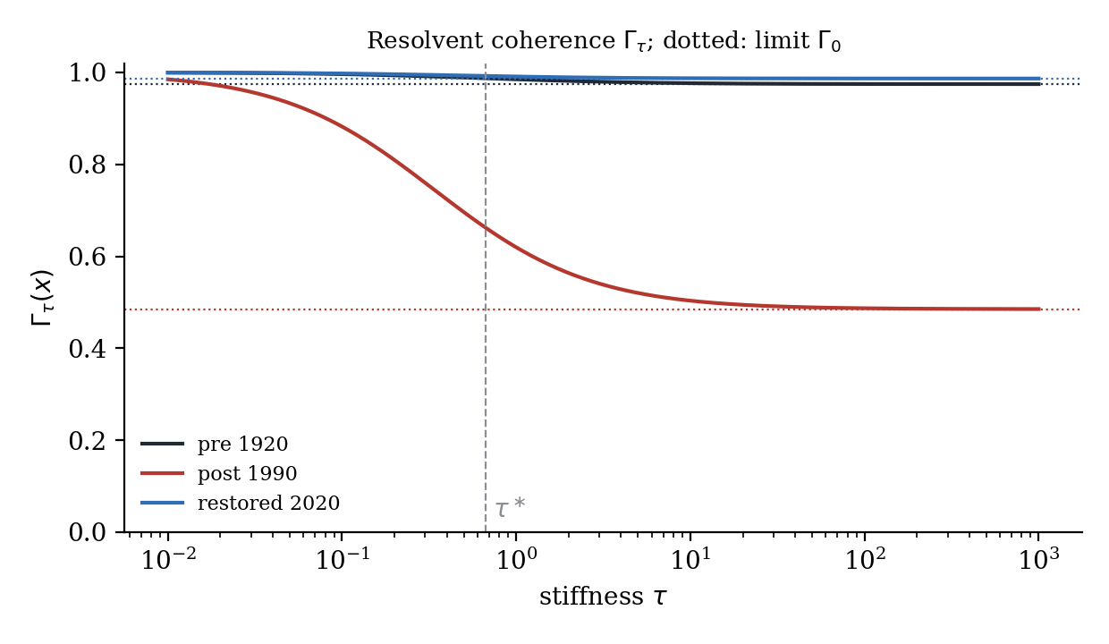
Setting. A path Wolves–Elk–Willows–Rivers with stalks $\mathbb R^2$ = (population health, behavioural regime) and identity maps, using the three v4.4 snapshots. Identity maps assert that adjacent trophic levels “should” report equal values. This is a placeholder for estimated maps (Section 2.6), kept for comparability [D].
| Snapshot | $E$ | $\|x\|^2$ | v4.4-style $1-R$ | $\Gamma_R$ | $\Gamma_0$ | $\Gamma_{\tau^\ast}$ |
|---|---|---|---|---|---|---|
| Pre-removal (c. 1920) | 0.20 | 4.32 | 0.954 | 0.986 | 0.975 | 0.987 |
| Post-removal (c. 1990) | 1.55 | 1.00 | −0.550 | 0.546 | 0.485 | 0.662 |
| Restored (c. 2020) | 0.08 | 2.81 | 0.972 | 0.992 | 0.987 | 0.992 |
Two corrections follow:
- v4.4 printed $\|x\|^2=3.83$ and $1.30$ for the first two snapshots and reported $\Gamma_{\text{post}}=-0.192$. The arithmetic is wrong, and the negative value is not “anti-coherence” in any case. It arises because $R(x)=E/\|x\|^2$ is a Rayleigh quotient that can exceed 1 whenever $\lambda_{\max}>1$. Every v5.0 measure lies in $[0,1]$ by construction (Proposition 5.3).
- The ordering pre < restored is within the range that measurement noise alone would produce for data of this precision (Proposition 5.10). It should not be read [E].
4.3 The clock ring: holonomy and its residue
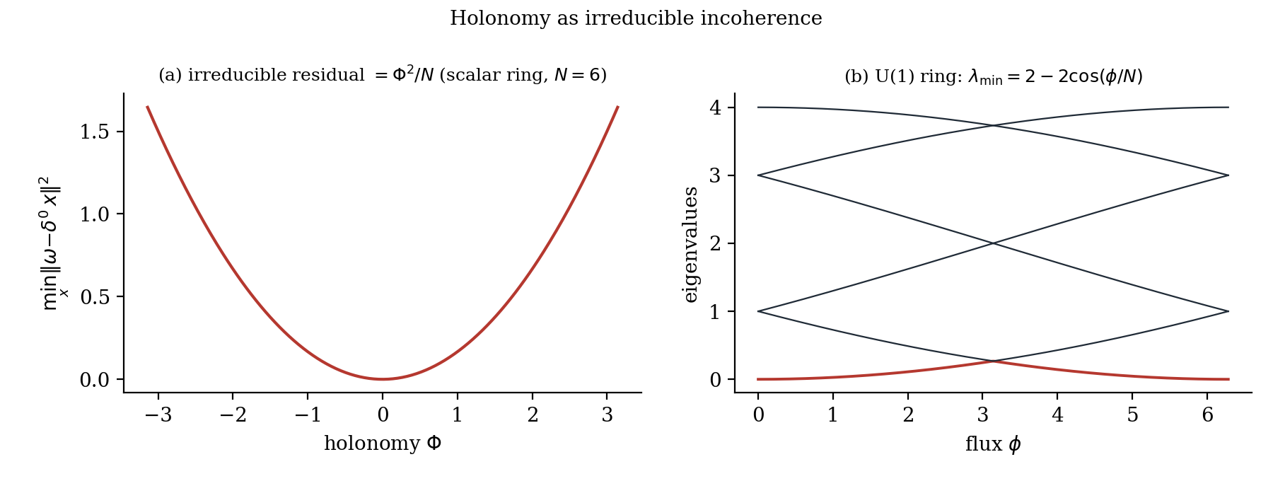
Setting. $N=6$ clocks on a ring. Each link measures the offset between neighbours, $\omega_e$, with stalks $\mathbb R$. The true offsets are a gradient, and a uniform holonomy $\Phi=0.6$ is added: $\omega=\delta^0t+\Phi/N$ [D].
Proposition 4.1 (Ring residual). On the scalar ring with $N$ edges and no face, every ω with holonomy $\Phi=\sum_e\omega_e$ satisfies $$\min_x\|\omega-\delta^0x\|^2=\Phi^2/N .$$ The residual is entirely harmonic.
Proof. On a cycle, $\operatorname{im}\delta^0=\{g:\sum_eg_e=0\}$, which has dimension $N-1$. The orthogonal complement is spanned by $\mathbf 1$. The projection of ω onto $\mathbf 1$ is $(\Phi/N)\mathbf 1$, with squared norm $\Phi^2/N$. With no faces there is no curl. ∎ [E]
Computed. The holonomy is 0.600 and $E_{\text{harm}}=0.0600=\Phi^2/N$. When the ring’s interior is declared a face, the same 0.0600 appears entirely as $E_{\text{curl}}$ and $E_{\text{harm}}=0$, as Proposition 3.7 requires. This is the result stated, for a gravitational ring, in The Dragged Frame (DRK-171) [E].
Proposition 4.2 (U(1) ring). Let each edge transport phases by $e^{i\phi/N}$, so that the holonomy is $e^{i\phi}$. The connection Laplacian has eigenvalues $$\lambda_k=2-2\cos\!\Big(\frac{2\pi k+\phi}{N}\Big),\qquad k=0,\dots,N-1 .$$ In particular $H^0=0$ unless $\phi\in2\pi\mathbb Z$.
Proof. The Fourier modes $x_j=e^{2\pi ikj/N}$ diagonalise the circulant connection Laplacian. ∎ [E]
For $\phi=1$ the computed spectrum is $\{0.0277,0.7265,1.3012,2.6988,3.2735,3.9723\}$, matching the closed form to $10^{-6}$. No global phase assignment exists ($b_0=0$), and the best attainable spectral coherence is $1-\lambda_{\min}/\lambda_{\max}=0.993$. This is the Aharonov–Bohm ring in sheaf form (Aharonov & Bohm 1959): a flux that is invisible locally on every link and unremovable globally [E].
4.4 The exchange complex: gradient, harmonic and curl together
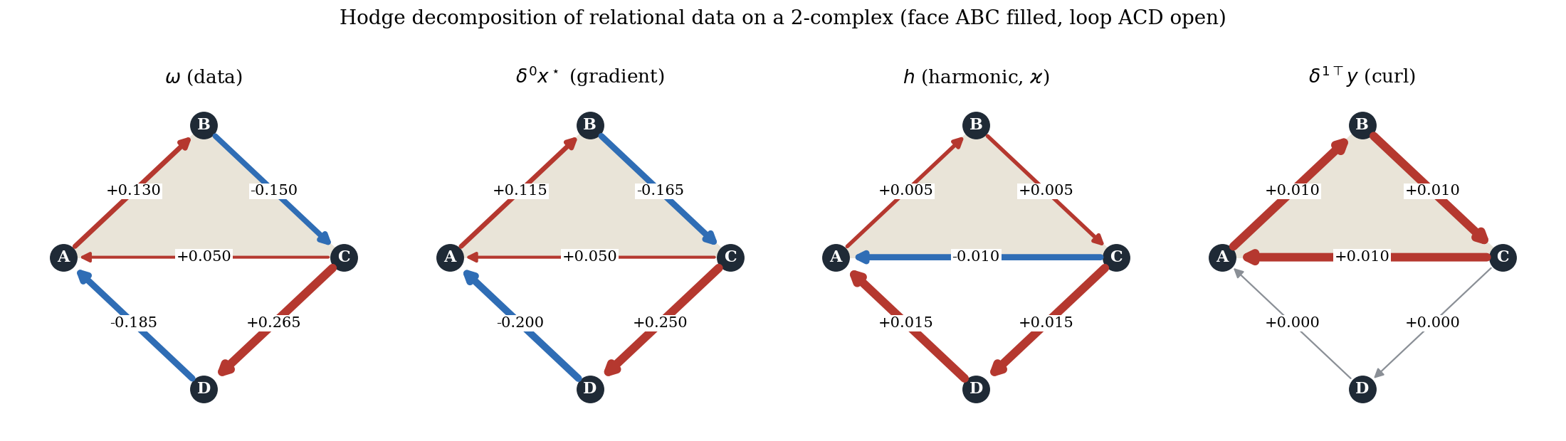
Setting. Four currencies A, B, C, D. Edge data are log exchange rates on A→B, B→C, C→A, C→D and D→A. The triangle ABC is declared a face, because its triangular cross-rates are quoted and checked; the loop ACD is not. The data are built from log prices $p=(0,0.10,-0.05,0.20)$, plus an arbitrage of 0.03 on A→B and a drift of 0.015 on each of C→D and D→A [D].
Computed.
| A→B | B→C | C→A | C→D | D→A | |
|---|---|---|---|---|---|
| ω | 0.130 | −0.150 | 0.050 | 0.265 | −0.185 |
| gradient | 0.115 | −0.165 | 0.050 | 0.250 | −0.200 |
| harmonic | 0.005 | 0.005 | −0.010 | 0.015 | 0.015 |
| curl | 0.010 | 0.010 | 0.010 | 0 | 0 |
- The curvature on ABC is 0.030, which is exactly the triangular arbitrage: the product of quoted rates around the triangle is $e^{0.03}$.
- $E_{\text{curl}}=3.0\times10^{-4}$, by projection and by Proposition 3.4.
- $E_{\text{harm}}=6.0\times10^{-4}$ and $\Gamma^1=0.994$; $b_0=b_1=1$.
- The periods of ω are 0.030 around A→C→D→A and 0.060 around A→B→C→D→A; they differ by the face curvature (Proposition 3.6). The harmonic part assigns the hole a single period, 0.040 [E].
Reading: an arbitrage inside a checked triangle is curvature, local and in principle detectable by anyone who quotes the triangle. A drift around an unchecked loop is a harmonic class, detectable only by someone who traverses the whole loop. The same market inconsistency is a “local scandal” or a “systemic hole” depending on what is jointly measured (Proposition 3.7) [D].
4.5 The toric code
Setting. The $L\times L$ square lattice on the torus, with qubits on edges. X-checks come from faces ($H_X=\partial_2^\top$) and Z-checks from vertices ($H_Z=\partial_1$), over $\mathbb F_2$ (Kitaev 2003; Dennis et al. 2002) [E].
Computed.
- $L=3$: $n=18$, $\operatorname{rank}\partial_1=\operatorname{rank}\partial_2=8$, so $k=n-8-8=2$.
- $L=4$: $n=32$, ranks 15 and 15, so $k=2$.
- In both cases the Euler characteristic is 0, and $k=\dim H_1(T^2;\mathbb F_2)=2$, with distance $d=L$ [E].
The commutation of all checks is $\partial_1\partial_2=0$: Lemma 2.5 over $\mathbb F_2$ [E].
4.6 Kuramoto synchrony is resolvent coherence
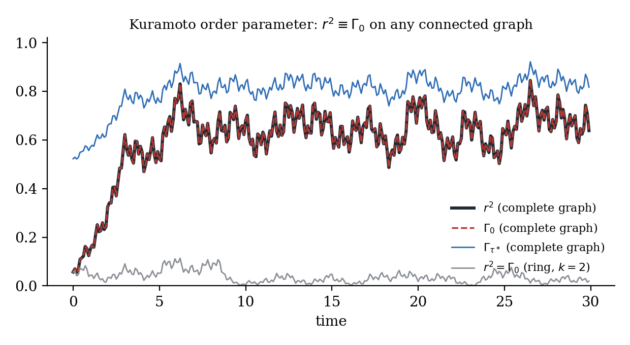
Proposition 4.3 (Order parameter). Let $G$ be any connected graph with the constant sheaf $\mathbb C$, and let $z_j=e^{i\theta_j}$. Then $$\Gamma_0(z)=r^2,\qquad r=\Big|\frac1N\sum_je^{i\theta_j}\Big| ,$$ where $r$ is the Kuramoto order parameter. On the complete graph, $$\Gamma_\tau(z)=r^2+\frac{1-r^2}{1+\tau N}.$$
Proof.
- Connectedness gives $H^0=\operatorname{span}(\mathbf 1)$.
- The projection is $Pz=(\bar z)\mathbf 1$, with $\bar z$ the mean.
- Hence $\|Pz\|^2=N|\bar z|^2=Nr^2$, while $\|z\|^2=N$, so $\Gamma_0(z)=r^2$.
- On the complete graph every nonzero eigenvalue equals $N$; substitute into the spectral form of $\Gamma_\tau$ (Proposition 5.3). ∎ [E]
Computed. For 40 Cauchy-distributed oscillators ($K=1.5$), simulated to $t=30$:
| Graph | max $\lvert r^2-\Gamma_0\rvert$ | final $r$ | final $\Gamma_{\tau^\ast}$ |
|---|---|---|---|
| Complete | $4\times10^{-16}$ | 0.799 | 0.817 |
| Ring, neighbours at distance 1 and 2 | $4\times10^{-17}$ | 0.141 | 0.600 |
On the ring, global synchrony fails while local phase agreement is high. $\Gamma_0$ (global) and $\Gamma_{\tau^\ast}$ (scale-limited) separate the two, which is what the stiffness τ is for (Section 5.2). This makes exact the claim in The Carrier and the Cargo (DRK-189) that $r$ is “the rank-1 shadow of Γ” [E/D].
4.7 Signed relations: structural balance as holonomy
Setting. A triangle of three agents. Each edge carries a sign $s_e\in\{\pm1\}$ (“ally/enemy”). The sheaf has stalks $\mathbb R$ and transports $x_v\mapsto s_ex_u$, i.e. an $O(1)$ connection [D].
Proposition 4.4 (Balance). On a connected graph with an $O(1)$ sheaf, $H^0\neq0$ if and only if every cycle has sign product $+1$. That is, the signed graph is balanced in Harary’s sense.
Proof. A nonzero global section is determined by its value at one vertex, propagated along a spanning tree. It is consistent on a non-tree edge if and only if the cycle that edge closes has trivial holonomy. ∎ (Harary 1953; Altafini 2013) [E]
Computed.
| Signs | Eigenvalues | $b_0$ | Reading |
|---|---|---|---|
| $(+,-,-)$, balanced | $\{0,3,3\}$ | 1 | A global section exists: two opposed camps with coherent values |
| $(+,+,-)$, unbalanced | $\{1,1,4\}$ | 0 | Frustration: no consistent assignment |
This corrects a claim in The Carrier and the Cargo (DRK-189, §6 ii) that “polarisation is a nonzero $H^1$ class” [E/D]:
- Polarisation into two internally coherent, mutually opposed camps is a global section of a balanced signed sheaf, i.e. bipartite consensus (Altafini 2013). It is an $H^0$ state.
- Fragmentation is disconnection: $b_0$ grows as edges are cut.
- Frustration, alliances that cannot be made consistent, is nontrivial holonomy. That is the genuine obstruction.
4.8 A cut that does not split
Setting. Take the ring of Example 4.3, $N=6$. Let $\mathcal E$ have stalks $\mathbb R^2$. On edge $k$, the head’s restriction map is the shear $\begin{pmatrix}1\&a_k\\0\&1\end{pmatrix}$ and the tail’s is the identity. Put $$a=(0.10,\,0.05,\,0,\,0.08,\,0.02,\,0.05).$$ The first coordinate is a constant subsheaf $\mathcal K$, and the quotient $\mathcal Q$ is the constant sheaf on the second coordinate. This is a short exact sequence (Definition 3.9) [D].
Computed. Take the global section $q\equiv1$ of $\mathcal Q$ and the stalkwise lift $e=(0,1)$ on every vertex. Then:
- $\delta_{\mathcal E}e$ has zero second coordinates, as Theorem 3.10 requires, and first coordinates $\omega_q=a$;
- the holonomy is $\sum_ka_k=0.30$;
- $E_{\text{harm}}(\omega_q)=0.0150=0.30^2/6$ and $E_{\text{curl}}=0$ (Proposition 3.11(i));
- the best lift found by direct least squares over all lifts has residual disagreement 0.0150 (Proposition 3.11(iv));
- $b_0(\mathcal E)=1$: the only global sections come from $\mathcal K$, so $q$ does not lift.
The shear is a “cut” whose re-gluing accumulates a twist of 0.30 around the loop [E].
4.9 The running example across the monograph
The institutional sheaf of Example 4.1 is the monograph’s running example. Every instrument is applied to the same data, so the measures can be compared on one object [D].
| Quantity | Value | Where |
|---|---|---|
| Disagreement energy $E$; $\lVert x\rVert^2$ | 1.84; 3.16 | Ex. 4.1 |
| Cohomology $b_0$, $b_1$ (cycle X–F–H) | 2, 2 | Ex. 4.1 |
| Spectral gap $\lambda_1^+$; relaxation time | 0.519; 1.93 cycles | Ex. 4.1, Thm. 15.1 |
| $\Gamma_{\tau^\ast}$ against no reference / against midpoint | 0.886 / 0.453 | Ex. 4.1, standard 5.7a |
| $\Gamma_0$; $\Gamma_R$; Jensen and gap bounds | 0.792; 0.860; [0.775, 0.957] | Prop. 5.4 |
| Most leveraged node (sensitivity) | HR (0.196) | Prop. 5.9 |
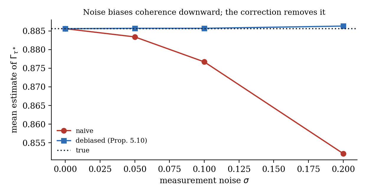
| Naive vs debiased Γ at noise σ = 0.2 | 0.852 vs 0.886 (true 0.886) | Prop. 5.10 |
| Agreement fraction $\sigma_{0.8}$ vs energy bound | 0.80 ≥ 0.425 | Prop. 5.11 |
| Repair map = Tweedie denoiser | agree to $3\times10^{-16}$ | Prop. 5.12 |
| Γ after deleting all relations | 1.000, with $b_1$ = 0 and $b_0$ = 10 | Thm. 19.2 |
| Compliance H→C, full and after one deletion | 2.667 → 4.000 → ∞ | Prop. 19.6 |
Read together, the rows say what the monograph says. The data have one structural hole (the X–F–H loop) and one dominant local disagreement (X–H). The score depends on the declared reference. Noise would make the institution look worse than it is. And the cheapest way to make it look perfect, deleting its relations, destroys the hole, splits the institution, and makes it unable to carry load [D].
Part II — Measures
5 Coherence Γ
The approved KO defines Γ as tracking “how well local sections glue into a globally consistent picture” (The Kaiju Manifesto, DRK-105). The corpus contains four inequivalent formulas for it:
- v4.4: $1-R$;
- Bootstrap Inception (DRK-185): $1-\|\delta s\|/\|s\|$;
- The Compressible Section (DRK-157): a dimension ratio;
- The Carrier and the Cargo (DRK-189): the order parameter.
This chapter fixes one canonical measure and derives the others as limits, bounds or special cases [D].
5.1 Definition
Definition 5.1 (Resolvent coherence). For vertex data $x\neq0$ and stiffness $\tau>0$, $$\Gamma_\tau(x)\;:=\;\frac{\big\langle x,\ (I+\tau L_{\mathcal F})^{-1}x\big\rangle}{\langle x,x\rangle}.$$ The default stiffness is $\tau^\ast:=\dim C^0/\operatorname{tr}L_{\mathcal F}$, the reciprocal mean eigenvalue. It is computed once on the reference base and then held fixed for every comparison (Axiom A2) [D].
Γ in v5.0 means $\Gamma_{\tau^\ast}$ unless another τ is declared [D].
Proposition 5.2 (Repair-cost form). $$\Gamma_\tau(x)=1-\frac{\mathcal C_\tau(x)}{\|x\|^2},\qquad \mathcal C_\tau(x):=\min_{y\in C^0}\Big\{\|y-x\|^2+\tau\,\langle y,L_{\mathcal F}y\rangle\Big\}.$$ The minimiser is $y^\ast=(I+\tau L)^{-1}x$.
Proof. Write $M=I+\tau L$, which is positive definite. Then $$\|y-x\|^2+\tau\langle y,Ly\rangle=\langle y,My\rangle-2\langle x,y\rangle+\|x\|^2 .$$ This is minimised at $y^\ast=M^{-1}x$, with minimum value $\|x\|^2-\langle x,M^{-1}x\rangle$. ∎ [E]
Reading: Γ is one minus the normalised cost of the cheapest coherent repair. The repair may change the data (cost $\|y-x\|^2$) or leave disagreement in place (cost $\tau E(y)$). The stiffness τ is the exchange rate between the two: the price of a unit of disagreement in units of a unit of data change. This is the resolvent (Tikhonov) smoother of graph signal processing (Shuman et al. 2013) applied to sheaves [E/D].
5.2 Spectral form, range and limits
Let $L=\sum_k\lambda_kP_k$ be the spectral decomposition, with $P_0$ the projector onto $\ker L=H^0$. Let $w_k=\|P_kx\|^2/\|x\|^2$, so that $\sum_kw_k=1$.
Proposition 5.3.
$\displaystyle \Gamma_\tau(x)=\sum_k\frac{w_k}{1+\tau\lambda_k}$.
$0\lt \Gamma_\tau(x)\le1$, with equality if and only if $x\in H^0$.
$\Gamma_\tau$ is non-increasing in τ, and $$\lim_{\tau\to\infty}\Gamma_\tau(x)=\Gamma_0(x):=\frac{\|P_0x\|^2}{\|x\|^2},\qquad \Gamma_\tau(x)=1-\tau R(x)+O(\tau^2)\ \ (\tau\to0),$$ where $R(x)=E(x)/\|x\|^2$.
Proof. (i) Diagonalise $M^{-1}$. (ii) Every term is positive; $\Gamma_\tau=1$ if and only if $w_k=0$ whenever $\lambda_k>0$. (iii) Each term $1/(1+\tau\lambda_k)$ is non-increasing in τ, tends to $\mathbf 1[\lambda_k=0]$, and has derivative $-\lambda_k$ at τ = 0. ∎ [E]
Γ_τ is therefore a spectral shape of the data: a low-pass filter whose cutoff is set by τ. Shape Is Spectrum (DRK-144) reads coherence as a distribution over a basis; in v5.0 the basis is the Laplacian eigenbasis and the reading is Proposition 5.3(i) [E/D].
The dial has three settings:
- Small τ measures only gross local disagreement.
- Large τ measures only global agreement ($\Gamma_0$).
- τ* sits at the system’s own mean scale.
The Kuramoto ring of Section 4.6 shows why the dial is necessary: high local agreement with no global synchrony gives $\Gamma_{\tau^\ast}=0.60$ and $\Gamma_0=0.02$ [E].
5.3 Bounds connecting the corpus’s formulas
Proposition 5.4. Let $\lambda_1^+$ and $\lambda_{\max}$ be the smallest nonzero and the largest eigenvalue. Then $$\max\Big\{\Gamma_0,\ \frac1{1+\tau R}\Big\}\ \le\ \Gamma_\tau\ \le\ \Gamma_0+\frac{1-\Gamma_0}{1+\tau\lambda_1^+},$$ $$1-\frac{R}{\lambda_1^+}\ \le\ \Gamma_0\ \le\ 1-\frac{R}{\lambda_{\max}}=:\Gamma_R .$$
Proof.
- $\Gamma_\tau\ge\Gamma_0$ because every term is non-negative and the $\lambda=0$ terms contribute $\Gamma_0$.
- $\Gamma_\tau\ge1/(1+\tau R)$ by Jensen’s inequality for the convex map $\lambda\mapsto(1+\tau\lambda)^{-1}$ under the weights $w_k$.
- The upper bound for $\Gamma_\tau$ replaces every nonzero eigenvalue by $\lambda_1^+$.
- For the second line, $R=\sum_{\lambda_k>0}w_k\lambda_k$ lies between $\lambda_1^+(1-\Gamma_0)$ and $\lambda_{\max}(1-\Gamma_0)$. ∎ [E]
How the corpus’s formulas relate to the canonical Γ:
- The spectral form $\Gamma_R$ (DRK-189’s “normalised” formula) is an upper bound on $\Gamma_0$.
- The unnormalised v4.4 form $1-R$ is not a coherence measure at all, since it is negative whenever $R>1$.
- DRK-185’s $1-\|\delta s\|/\|s\|=1-\sqrt{R}$ is a monotone transform of $R$ with the same defect.
All three are retired as headline measures; $\Gamma_R$ is retained as a computable bound [D].
5.4 Invariances and the reporting duty
Proposition 5.5.
$\Gamma_\tau(cx)=\Gamma_\tau(x)$ for every $c\neq0$.
$\Gamma_{\tau/a}(x;aL)=\Gamma_\tau(x;L)$ for every $a>0$. Hence $\Gamma_{\tau^\ast}$ is invariant under rescaling every restriction map by the same factor.
If $Q$ is a block-orthogonal change of stalk bases, with restriction maps transformed accordingly, then $\Gamma_\tau(Qx;QLQ^\top)=\Gamma_\tau(x;L)$.
Proof. (i) and (ii) are immediate from Definition 5.1, and $\tau^\ast$ scales as $1/a$. For (iii), $(I+\tau QLQ^\top)^{-1}=Q(I+\tau L)^{-1}Q^\top$. ∎ [E]
Part (iii) is the precise form of “coherence does not depend on how each node labels its own coordinates”. It underlies the drift prediction of Chapter 20 [E/D].
Proposition 5.6 (Monotonicity in the relations). Fix τ. If $L\preceq L'$ in the Loewner order, then $\Gamma_\tau(x;L')\le\Gamma_\tau(x;L)$ for every $x$. In particular:
- adding an edge, with any restriction maps, never raises Γ_τ;
- deleting an edge never lowers it;
- deleting every edge gives $\Gamma_\tau\equiv1$.
Proof. $L\preceq L'$ implies $I+\tau L\preceq I+\tau L'$, and matrix inversion is order-reversing on positive-definite matrices. Adding an edge adds the positive semidefinite term $\delta_e^\top\delta_e$. ∎ [E]
Proposition 5.6 is the engine of the anti-totalisation theorem (Chapter 19). It also corrects v4.4’s “false overlap” signature (Chapter 18) [D].
Proposition 5.7 (Global-section inflation). For $s\in H^0$, $s\ne0$: $$E(x+cs)=E(x)\ \ \text{for all }c,\qquad\text{and}\qquad \Gamma_\tau(x+cs)\to1\ \ (c\to\infty).$$
Proof. $\delta^0s=0$, and the $H^0$ weight $w_0\to1$. ∎ [E]
Reporting standard 5.7a. Γ must always be reported with:
- the energy $E$;
- the declared reference $x_{\text{ref}}$ against which data are measured;
- the stiffness τ;
- the complex, stalks and restriction maps.
Example 4.1 shows a single dataset scoring 0.886 or 0.453 depending on the reference. A Γ reported alone is not admissible evidence [D].
5.5 Coherence is not soundness
Proposition 5.8 (Blindness to coherent error). Let $x=x_{\text{true}}+s$ with $s\in H^0$. Then $\delta^0x=\delta^0x_{\text{true}}$, so every function of the disagreements takes the same value on the true state and on the falsified one.
Now let anchors be added: cells $a$ carrying fixed reference data $r_a$, linked to vertices by restriction maps that together form an operator $A$. Then the falsification $s$ is detectable if and only if $As\neq0$. The undetectable subspace $$\mathcal U:=H^0\cap\ker A$$ can only shrink as anchors are added [E].
Proof. The first statement is Lemma 2.5 applied to $\delta^0s=0$. With anchors, the anchor residual $Ax-r$ changes by $As$. Adding anchors adds rows to $A$, which shrinks $\ker A$. ∎ [E]
This is the formal core of three corpus results:
- “the synchronised lie” (The Carrier and the Cargo, DRK-189, §7);
- the honest referee of 知行合一: When Automation Removes the Only Honest Referee (DRK-131);
- abduction’s “coherent-but-unsound” section (The Guessed Section, DRK-170).
A system can be perfectly coherent and entirely wrong. Only restriction maps to something outside the system’s own sections, the anchors, can tell [E/D].
5.6 Estimation
Proposition 5.9 (Gradient and error propagation). With $M=I+\tau L$, $$\nabla_x\Gamma_\tau=\frac{2}{\|x\|^2}\big(M^{-1}x-\Gamma_\tau(x)\,x\big).$$ For measurement error with covariance $\Sigma_x$, the delta method gives $\sigma^2_\Gamma\approx\nabla\Gamma^\top\Sigma_x\nabla\Gamma$. The node-wise norms of $\nabla\Gamma$ rank nodes by their leverage over the score, which is also the order in which a manipulator would attack them [E].
Proof. Apply the quotient rule to $\langle x,M^{-1}x\rangle/\langle x,x\rangle$, using the symmetry of $M^{-1}$. ∎
Proposition 5.10 (Noise bias and its correction). Let $\tilde x=x+\eta$ with $\mathbb E\eta=0$ and $\operatorname{Cov}\eta=\Sigma$. Then for every symmetric $B$, $$\mathbb E\big[\langle\tilde x,B\tilde x\rangle\big]=\langle x,Bx\rangle+\operatorname{tr}(B\Sigma).$$ In particular:
- the measured energy is inflated by $\operatorname{tr}(L\Sigma)$;
- the naive $\Gamma_\tau$ is biased toward lower coherence;
- the ratio estimator $$\widehat\Gamma_\tau=\frac{\langle\tilde x,M^{-1}\tilde x\rangle-\operatorname{tr}(M^{-1}\Sigma)}{\|\tilde x\|^2-\operatorname{tr}\Sigma}$$ is a ratio of unbiased estimators of the numerator and denominator, and is consistent as $\Sigma\to0$ or under averaging of repeated measurements.
Proof. $\mathbb E\langle\eta,B\eta\rangle=\operatorname{tr}(B\Sigma)$, and the cross terms vanish because $\mathbb E\eta=0$. ∎ [E]
Computed (institutional data, isotropic noise, 20,000 replicates):
| σ | mean $E$ (predicted) | naive $\Gamma_{\tau^\ast}$ | debiased | true |
|---|---|---|---|---|
| 0 | 1.840 (1.840) | 0.886 | 0.886 | 0.886 |
| 0.05 | 1.889 (1.890) | 0.883 | 0.886 | 0.886 |
| 0.10 | 2.043 (2.040) | 0.877 | 0.886 | 0.886 |
| 0.20 | 2.646 (2.640) | 0.852 | 0.886 | 0.886 |
Noisy institutions look less coherent than they are. A coherence decline that is not larger than the noise inflation predicted by Proposition 5.10 is not evidence of decline [E/D].
5.7 The other coherence quantities
| Symbol | Definition | Status |
|---|---|---|
| $\Gamma_{\tau}$ | Definition 5.1 | Canonical vertex coherence |
| $\Gamma_0$ | $\|P_{H^0}x\|^2/\|x\|^2=\lim_{\tau\to\infty}\Gamma_\tau$ | Global agreement share. Discontinuous in the restriction maps: generic perturbations give $H^0=0$, so it is reported only for exactly specified sheaves |
| $\Gamma_R$ | $1-R/\lambda_{\max}$ | Spectral upper bound on $\Gamma_0$ (Prop. 5.4) |
| $\Gamma^1$ | $E_{\text{grad}}/\|\omega\|^2$ | Integrability share of relational data (Def. 3.2a) |
| $\Gamma_{\text{top}}$ | $b_0/(b_0+b_1)$ | Structural index of the sheaf alone (The Compressible Section, DRK-157); data-free |
| $r^2$ | Kuramoto | Equal to $\Gamma_0$ for unit phasors on a connected graph (Prop. 4.3) |
| $\sigma$, $T$ | Fraction of agreeing edges or overlaps (DRK-142, DRK-139) | $\ell^0$ coherence: well-posedness check, syndrome complement; not headline (Prop. 5.11) |
v4.4’s estimator programme (sampling protocol, uncertainty propagation, adversarial robustness) is now carried by the reporting standard 5.7a and Propositions 5.9–5.10 [D].
Agreement counts. The corpus contains two counting measures:
- the cocycle density $\sigma(\mathcal F)=\frac1{|E|}\sum_e\chi(e)$, where $\chi(e)=1$ if edge $e$ glues cleanly (Wrestling with God, DRK-142);
- taxamhet $T(\mathcal F)$, the fraction of overlaps on which two local classifications agree on the type of object, proposed as the “zeroth-order diagnostic, prior to Γ” (The Welcomed Section, DRK-139; The Finite Sheaf, DRK-141).
Both are $\ell^0$ coherences. They count edges and ignore the size of the disagreement.
- $T$ is σ for sheaves whose stalks are finite sets of types.
- $1-\sigma$ is the normalised weight of the syndrome, the “fraction of violated checks” in the soundness inequality of Section 9.2.
The two families are linked as follows [E/D].
Proposition 5.11 (Counting versus energy). For a tolerance $\varepsilon>0$, let $\sigma_\varepsilon$ be the fraction of edges with $\|(\delta^0x)_e\|\le\varepsilon$. Then $$\sigma_\varepsilon\ \ge\ 1-\frac{E(x)}{|E|\,\varepsilon^2}.$$ Exact agreement ($\varepsilon=0$) is not controlled by $E$ at all. It is discontinuous in the data, and it can be inflated by fabricated agreeing edges (§18.2).
Proof. At most $E/\varepsilon^2$ edges can carry squared disagreement greater than $\varepsilon^2$, by Markov’s inequality applied to the edge energies. ∎ [E]
Computed (institutional sheaf, $\varepsilon=0.8$): $\sigma_{0.8}=0.80$, against a guaranteed lower bound of 0.425 [E].
Reading: T and σ answer a different question from Γ. Γ asks how much repair coherence costs. T and σ ask whether the stalks share a type space at all; if they do not, restriction maps are undefined and no Γ can be computed. They are retained as the well-posedness check that precedes Γ, and as the discrete side of soundness. They are not admissible as headline coherence [D].
5.8 The repair is a posterior mean
The resolvent of Definition 5.1 has an exact probabilistic reading. That reading connects Γ to Gaussian Markov random fields and to the denoisers of diffusion models (§15.6) [E].
Proposition 5.12 (Bayesian and score form). Give the signal $y\in C^0$ the intrinsic Gaussian Markov random field prior with precision $\tau L_{\mathcal F}$: $$p(y)\propto\exp\!\big(-\tfrac\tau2\langle y,Ly\rangle\big),$$ flat on $H^0$ (Rue & Held 2005). Observe $x=y+\xi$ with $\xi\sim\mathcal N(0,I)$. Then:
$\mathbb E[y\mid x]=(I+\tau L)^{-1}x$, the repair $y^\ast$ of Proposition 5.2. Hence $$\Gamma_\tau(x)=\frac{\langle x,\ \mathbb E[y\mid x]\rangle}{\|x\|^2},$$ and the repair cost $\mathcal C_\tau(x)$ is twice the minimum of the negative log-posterior, up to an additive constant.
Tweedie’s formula holds in the form $\mathbb E[y\mid x]=x+\nabla_x\log p(x)$, with $p$ the marginal density of the observation on the non-global modes (Efron 2011).
The disagreement energy is a log-density: $E(x)=-\tfrac2\tau\log p(x)+\text{const}$ under the prior.
Proof.
The posterior precision is $I+\tau L$ and the posterior mean is $(I+\tau L)^{-1}x$. On $H^0$ the prior precision is zero, so the mean equals the data there.
In each eigenmode with $\lambda_k>0$, the marginal variance is $1+(\tau\lambda_k)^{-1}$. Then $$x_k-\frac{x_k}{1+(\tau\lambda_k)^{-1}}=\frac{x_k}{1+\tau\lambda_k},$$ which is the resolvent.
Take the logarithm of the prior. ∎
The script confirms (i)–(ii) to $3\times10^{-16}$ [E].
Three consequences connect this to the rest of the monograph:
- Γ is a model-based quantity. It measures how much of the data survives the best estimate under the prior that disagreement is improbable. τ is the prior’s precision, which is why Axiom A2 fixes it.
- The noise correction of Proposition 5.10 and the noise floor of Proposition 18.1 are Gaussian-model statements of the same kind, and they apply under the same assumptions.
- The repair step and the denoising step of a score-based generative model are one operation when the prior is sheaf-structured (§15.6).
[E/D]
6 Narrative Self-Reference Ψ and Grounding
6.1 Definition
The approved KO defines Ψ as “the ratio of narrative self-reference to reality-contact” (The Kaiju Manifesto, DRK-105). Its “psychosis metric” label is retired; the measure is structural, not clinical [D].
The operational form follows v4.4.
- $N_S$ is the finite set of claims a system asserts in a declared corpus. A claim is an element of $N_S$; nothing outside $N_S$ is scored.
- $O_S$ is a set of external observations, disjoint from $N_S$.
- Each claim $c\in N_S$ has an evidential support $\operatorname{supp}(c)\subseteq N_S\cup O_S$, assigned by the protocol of §6.5.
Define $$n_{\text{self}}=|\{c\in N_S:\operatorname{supp}(c)\subseteq N_S\}|,\qquad n_{\text{contact}}=|\{c\in N_S:\operatorname{supp}(c)\cap O_S\ne\emptyset\}|,\qquad \Psi=\frac{n_{\text{self}}}{n_{\text{contact}}}.$$ Unsupported claims, with empty support, count as self-referential [D].
Lemma 6.1. Under these definitions $n_{\text{self}}+n_{\text{contact}}=|N_S|$. Hence Ψ is the odds of self-support, $$\Psi=\frac{\bar\psi}{1-\bar\psi}\in[0,\infty],\qquad \bar\psi:=\frac{n_{\text{self}}}{|N_S|}=\frac{\Psi}{1+\Psi}\in[0,1].$$
Proof. Each $c\in N_S$ falls in exactly one class. Either $\operatorname{supp}(c)\subseteq N_S$, or it contains an element outside $N_S$. Since supports lie in $N_S\cup O_S$, that element is in $O_S$. The two cases are exclusive because $N_S\cap O_S=\emptyset$. ∎ [E]
The bounded companion $\bar\psi$ reconciles the corpus’s usage:
- “Ψ → 1” in The Protocol and the Predator (DRK-133, KO kayfabe) and in Ouroboros Debt (DRK-176) is read as $\bar\psi\to1$: almost every claim is supported only by other claims.
- Ψ itself is unbounded and diverges in the same limit. Thresholds $\Psi_{\text{viable}}$ are stated in odds [D].
6.2 The grounding sheaf
Build a support complex:
- vertices: claims;
- edges: support relations between claims, carrying restriction maps that encode what one claim implies about another;
- anchors: observations in $O_S$, attached to the claims they support.
Self-supported claims are those with no path to an anchor. By Proposition 5.8, the falsifications of the narrative that are invisible to every check, internal or external, form $\mathcal U=H^0\cap\ker A$. Adding anchors shrinks $\mathcal U$ [E/D].
Hypothesis H6.1. In observed narratives, the undetectable share $\dim\mathcal U/\dim H^0$ increases with $\bar\psi$. Ψ is then an inexpensive observable proxy for the dimension of the space of coherent lies a system could hold without internal or external alarm [H].
6.3 Ψ and Γ are independent coordinates
v4.4 conjectured that Ψ and Γ are inversely monotone (its §4.1.2). Proposition 5.8 refutes the conjecture as a law. A system can raise Γ toward 1 by adding a coherent narrative, a global section, while $\bar\psi$ rises, because nothing in Γ consults the anchors. Functional independence, meaning that neither measure determines the other, is therefore proved [E]. Whether the two are statistically correlated in real systems is a separate, empirical question [H]. The conjecture is withdrawn as a law [D].
What replaces it is a two-coordinate diagnostic:
| low $\bar\psi$ (grounded) | high $\bar\psi$ (self-referential) | |
|---|---|---|
| high Γ | Coherent and accountable | Kayfabe / synchronised lie / egregore: locally glued, globally unanchored |
| low Γ | Honest disagreement; repairable | Fragmenting self-narratives |
The dangerous quadrant is the upper right:
- Kayfabe (KO, DRK-133) names it in the working vocabulary.
- An egregore (KO, The Compressed Will, DRK-191) is “a well-glued section whose stability no longer depends on any single stalk” (a global section maintained by the gluing itself rather than by anchors) [D].
Whether the empirical joint distribution of (Γ, $\bar\psi$) concentrates off the anti-diagonal is an open question (Prediction P1′, Chapter 22) [H].
6.4 Observer-level self-reference
The KO synchronicity density σ(t) (The Common Base, DRK-177) is “the fraction of salient events at time t that the observer reads as addressed to the self”. It is the observer-level analogue of $\bar\psi$: interpretation supported only by self-reference [D].
Its methodological companion is base-rate hygiene. With $N\approx10^6$ salient events in 35 days and coincidence probability $p\approx10^{-6}$, the expected number of “unreasonable” coincidences is $Np\approx1$ per month (computed in DRK-177; the one-event-per-month heuristic is the conventional gloss on Littlewood’s Miscellany (Littlewood 1986), not a theorem in it). A σ(t) excess must be computed against such a base rate before it is read [E/D].
The The Ouroboros Debt (DRK-176) basin share $\beta_{\text{self}}=\mu(B(A_{\text{self}}))/\mu(X)$ is renamed from Ψ to $\beta_{\text{self}}$. It is the dynamical analogue: the share of state space that flows into the self-model’s attractor. A monotone relation between $\beta_{\text{self}}$ and $\bar\psi$ is hypothesised, not derived [H].
6.5 Coding protocol for Ψ
Ψ is measurable only under a protocol a second person can apply. v5.0 specifies the following minimum [D].
- Corpus. Declare the documents, the period and the issuing system $S$ in advance.
- Claim unit. A claim is a declarative clause asserting a proposition about $S$ or its situation that could in principle be false. Questions, commands, hedged speculation and pure evaluation without a factual component are excluded. Each claim is entered once; repetitions are de-duplicated by meaning.
- Support assignment. $\operatorname{supp}(c)$ is everything the text itself offers as evidence for $c$: explicit citations, references, data, quotations and inferential markers (“because”, “as shown by”) within the same paragraph or a referenced appendix.
- Each item is coded internal if it is another claim, statement or document of $S$ itself.
- Each item is coded external if it is an independently produced observation: third-party data, measurements, audited records or independent reports.
- Mixed items are split. Nothing outside the text is used.
- Reliability. Two coders code a random 20% sample independently. Ψ is reported only if Cohen’s κ ≥ 0.70 on the internal/external decision (Landis & Koch 1977). Otherwise the codebook is revised and the sample recoded.
- Uncertainty. Report $\bar\psi$ with a bootstrap interval over claims, and Ψ derived from it.
Automated coding (NLP extraction of claims and support) is admissible only after it reaches κ ≥ 0.70 against the human coders on the same sample. Until a corpus has been coded this way, the computable debt in this monograph is $K_\Gamma$ (§7.3), not $K$ [D].
7 The Debt Calculus
7.1 One functional, four debts
The corpus contains several integrals called “debt”. They share one form.
Definition 7.1 (Ratchet functional). For a locally integrable rate $f:[0,T]\to\mathbb R$ and a bounded weight $w\ge0$, $$\mathcal D[f,w](t):=\int_0^t\big[f(s)\big]^+\,w(s)\,ds,\qquad [a]^+=\max(a,0).$$
Proposition 7.2. $\mathcal D$ has the following properties:
$\mathcal D(0)=0$, and $\mathcal D$ is non-decreasing and absolutely continuous.
It is additive over consecutive intervals.
$\mathcal D[f,w](t)=0$ if and only if $f\le0$ almost everywhere on $\{w>0\}\cap[0,t]$.
It is monotone in $f$ and positively homogeneous.
It is subadditive: $\mathcal D[f+g,w]\le\mathcal D[f,w]+\mathcal D[g,w]$.
Proof. (i)–(iv) are properties of the Lebesgue integral of a non-negative integrand. (v) follows from $[a+b]^+\le[a]^++[b]^+$. ∎ [E]
Subadditivity has a reading. Splitting one excess into two cannot increase the debt, and two excesses that partly cancel accrue less debt together than apart. Debt penalises net excess at each instant, not gross activity [E/D].
The canonical instances.
| Debt | Rate $f$ | Weight $w$ | Defined in | KO |
|---|---|---|---|---|
| Coherence debt $K(t)$ | $\Psi(t)-\Psi_{\text{viable}}$ | irreversibility $w(t)$ | v4.4 eq. (7.1); The Coherence Debt (DRK-121) | K(t) |
| Trophic debt $\Theta(t)$ | $-\dot{\mathcal V}_{\text{exo}}(t)$ | 1 | Ouroboros Debt (DRK-176) | Θ |
| Stage deficit $D_k(t)$ | $C_k(t)-R_k(t)$ | 1 | The Earth Engine (DRK-193) | (earth engine) |
| Dietary debt $K_{\text{diet}}(t)$ | $\mathrm{HTL}(t)-\mathrm{HTL}_{\text{viable}}$ | $w(t)$ | The Komodoburger Franchise (DRK-136) | — |
All four are ratchets in the sense of Definition 7.1, so Proposition 7.2 applies to each without further proof [E]. Whether they measure the same underlying quantity is a separate, empirical question (Hypothesis H7.3) [H].
7.2 Gross debt and outstanding balance
v4.4 said both that K “accumulates monotonically” and that it “can only be reduced through structural intervention”. As written, K is monotone by construction and cannot be reduced at all. v5.0 resolves this by separating two quantities [D]:
- $K(t)$ is the gross accrued debt, monotone.
- The outstanding balance is $$B_K(t):=K(t)-P_K(t),$$ where $P_K$ is the non-decreasing cumulative discharge recorded at correction events: reforms, reintroductions, repairs, or (in the code picture of Section 12.3) decoder corrections.
Two diagnostics follow. A system with high $K$ and low $B_K$ has paid its bills. A system with high $B_K$ is running a deficit that, on the Draken reading, is discharged eventually. The discharge is either deliberate or forced by a correction event, which Ouroboros Debt (DRK-176) models as a basin-boundary metamorphosis (Grebogi, Ott & Yorke 1987) [D].
7.3 Quantities renamed out of the debt family
Three corpus integrals are not ratchets and are renamed so that “debt” has one meaning [D]:
| Old usage | New name | Formula | Why it is not a debt |
|---|---|---|---|
| “K” in The Substrate and the Game (DRK-130) | accumulated incoherence $I(t)$ | $\int_0^t\|\delta^0x(s)\|\,ds$ | Not thresholded; any nonzero disagreement accrues |
| “K” in The Finite Sheaf (DRK-141) | claim–measurement gap $G(t)$ | $\int_0^t(\Gamma_{\text{claimed}}-\Gamma_{\text{measured}})\,ds$ | Signed; can decrease |
| “K” in Ouroboros Debt (DRK-176) | curvature load $C(t)$ | $\int_0^t\|\delta^1\omega(s)\|\,ds$ | A load from curvature (Prop. 3.4), not an excess over a threshold |
The positive part of the claim–measurement gap, $K_\Gamma:=\mathcal D[\Gamma_{\text{claimed}}-\Gamma_{\text{measured}},1]$, is a ratchet. It is the most directly measurable instance of the K-family, because it needs no NLP pipeline for Ψ, only a reported coherence and a measured one [D].
7.4 Debt and obstruction
Hypothesis H7.1 (Masked obstruction). Coherence debt accrues fastest when a system reports an obstruction as resolved. That is, $\dot K$ is bounded below by a positive multiple of $E_{\text{obs}}$ whenever $\Gamma_{\text{claimed}}>\Gamma_{\text{measured}}$. Irreducible disagreement that is acknowledged costs maintenance. Irreducible disagreement that is denied accrues debt [H].
The toric code gives the most literal model of silent accrual. An error string of length ℓ produces a syndrome of weight 2 regardless of ℓ. Damage therefore grows below the reporting surface until it crosses $d/2$ and is “settled” all at once by a wrong correction (The Warded Class, DRK-190, §7) [E/D]. In debt terms, the balance $B_K$ grows invisibly whenever the system’s checks have low soundness (Section 9.3) [D].
Hypothesis H7.2 (Co-divergence). As $\bar\psi\to1$, $\dot K$ and $\dot\Theta$ diverge together. Coherence debt is the epistemic bill and trophic debt the metabolic bill of the same closed loop (Ouroboros Debt, DRK-176) [H].
Hypothesis H7.3 (Unity of debts). The stage deficit $D_k$ is an instance of Θ, i.e. over-consumption of a stage destroys exogenous variety. The Earth Engine (DRK-193) leaves this open; so does v5.0 [H].
Hypothesis H7.4 (Subsidised pathology). Let $S$ be the trophic surplus (intake minus maintenance). The maximum sustainable self-reference increases with accumulated surplus: $\bar\psi^{\text{sust}}_{\max}=g\big(\int_0^tS\,ds\big)$ with $g'>0$. An energy-rich system can carry a deeper self-model further from reality before correction (Ouroboros Debt, DRK-176) [H].
7.5 Care and variety
The care operator (Norm N2) needs a variable.
Let $\mathcal V$ be variety: the logarithm of the number of distinguishable states of a system (Ashby 1956), estimated operationally as the Shannon entropy of its observed state distribution. Following The Countable Mouth (DRK-181), split its rate of change as $$\dot{\mathcal V}=\dot{\mathcal V}_{\text{endo}}+\dot{\mathcal V}_{\text{exo}}:$$ [D]
- $\dot{\mathcal V}_{\text{endo}}$ is variety generated within the system (mutation, invention);
- $\dot{\mathcal V}_{\text{exo}}$ is the change the agent causes in the variety of what it is coupled to [D].
The approved KO states care as $\dot{\mathcal V}_{\text{exo}}=0$ (The Bridge and the Burn, DRK-162). Ouroboros Debt (DRK-176) writes the care condition as $\dot{\mathcal V}_{\text{exo}}\ge0$. v5.0 reconciles the two as follows [D]:
- Care is the zero-contribution constraint. The agent neither destroys nor homogenises what it is bound to; this covers imposing its own form on others, which raises its share of their state while lowering their variety.
- Accounting is asymmetric. Only the destructive side accrues trophic debt, $\Theta=\mathcal D[-\dot{\mathcal V}_{\text{exo}},1]$.
The optimisation axiom N1 constrains the system’s own diversity ($dH/dt\ge0$). N2 constrains its effect on others’ variety. Together they forbid both self-simplification and export of simplification [D].
8 Abstraction Depth α
Definition 8.1 (Path abstraction depth). For a path $\gamma=v_0\to v_1\to\dots\to v_k$ in the support or command complex, $$\alpha(\gamma)=\sum_{i=0}^{k-1}\Big(1-\cos\angle\big(\rho_{v_ie_i}x_{v_i},\ \rho_{v_{i+1}e_i}x_{v_{i+1}}\big)\Big),$$ with the convention $\cos\angle(\cdot,0)=0$. This is the v4.4 formula. Each term lies in $[0,2]$ and measures how much meaning is lost or turned across one representational hop [D].
v4.4 noted that α is path-dependent. v5.0 removes the dependence.
Definition 8.2. $\alpha^\ast(u,v):=\min_{\gamma:u\to v}\alpha(\gamma)$.
Proposition 8.3. $\alpha^\ast$ is well defined on a finite connected complex, computable by Dijkstra’s algorithm, symmetric when the edge terms are symmetric, and satisfies the triangle inequality $\alpha^\ast(u,w)\le\alpha^\ast(u,v)+\alpha^\ast(v,w)$.
Proof. The edge weights are non-negative and the graph is finite. A concatenation of paths is a path. ∎ [E]
The individual edge weights $1-\cos$ do not satisfy a triangle inequality. Only the minimal-path form is a pseudometric, and only it should be compared across systems [E/D].
Approved KO. Abstraction depth is “the number of representational layers between a claim to power and the capacity that underlies it” (Abstraction Depth, DRK-108). $\alpha^\ast$ from the claim vertex to the capacity vertex is its weighted, path-independent measurement [D].
Prediction (P3, retained). Across institutions with comparable complexes, $\alpha^\ast$ from claim to capacity correlates positively with time-to-correction after a falsifying event [H].
The v4.4 historical table, which assigned α from 0 for varanid combat to 7–10 for the attention economy, is retained in the companion volume as an illustrative ordering, not a measurement [H].
9 The Invariant and the Warded Triple
9.1 Metrics versus invariant
The Invariant (DRK-175) distinguishes two species of quantity:
- metrics (Γ, Ψ, K): continuous, frame-dependent energy functionals;
- the invariant ϰ: discrete, preserved under deformation that does not change the base.
The Hodge spine makes the distinction exact. Metrics are norms of projections. ϰ is a cohomology class, invariant under gauge (Proposition 3.3) and changed only by changing the complex (Proposition 3.7) [E/D].
The coherence genus is $b_1=\dim H^1$, the number of independent irreducible ways local relations fail to integrate. For the constant sheaf $\mathbb R^d$ on a graph, $$b_1=d\,(|E|-|V|+c),$$ where $c$ is the number of components [E].
On the justification offered in DRK-175 for calling ϰ the invariant:
- The linking number of two curves is an $H^1$ pairing: the class of one curve in $H_1$ of the other’s complement, by Alexander duality (Hatcher 2002) [E].
- The Jones polynomial and Chern–Simons invariants (Witten 1989) are not degree-1 cohomology classes, and Chern numbers live in $H^2$ (Thouless et al. 1982).
The analogy to knot theory therefore holds for linking but not beyond it. The v5.0 claim is limited accordingly [E/D].
9.2 The warded triple
The approved KO (The Warded Class, DRK-190) proposes $$\mathfrak W(\mathcal F):=(b_1,\ d,\ \rho_s):$$
- the rank $b_1$;
- the (co)systole $d$: the least weight of a cocycle that is not a coboundary, i.e. how much local damage flips a class;
- the soundness $\rho_s$: whether local checks register damage in proportion to its size.
The KO writes soundness as ρ. v5.0 writes $\rho_s$ to keep ρ for restriction maps (Appendix A) [D].
DRK-190, §9, identifies a gap: $d$ and $\rho_s$ need a weight on real cochains before they can be measured on Draken sheaves. v5.0 closes the gap for soundness [D].
Proposition 9.1 (Spectral soundness). For every $f\in C^1(X;\mathcal F)$ over $\mathbb R$, $$\|\delta^1f\|\ \ge\ s_1\cdot\operatorname{dist}(f,Z^1),\qquad s_1:=\sqrt{\lambda^+_{\min}(\Delta^2)},$$ where $Z^1=\ker\delta^1$ and $\lambda^+_{\min}$ is the smallest nonzero eigenvalue. The constant is sharp.
Proof.
- By Theorem 3.1, $f-\Pi_{Z^1}f=\Pi_{\text{curl}}f\in\operatorname{im}\delta^{1*}=(\ker\delta^1)^\perp$.
- On that subspace, $\|\delta^1v\|\ge s_1\|v\|$, where $s_1$ is the smallest nonzero singular value of $\delta^1$.
- Equality holds for the corresponding singular vector. ∎ [E]
$s_1$ is the ℓ²-analogue of the coboundary-expansion constant of Linial & Meshulam (2006) and Gromov (2010), as reported in DRK-190 [E/D]:
- a sheaf with $s_1$ bounded below raises alarm in proportion to damage;
- $s_1\to0$ is silent drift.
The systole $d$ remains defined only over $\mathbb F_2$ (codes), or over a declared integer lattice of periods. A real-valued instrument for $d$ is an open problem [D].
9.3 Regimes
The regime table of DRK-190, §8, restated with the spectral instrument [D]:
| Regime | Signature | Reading |
|---|---|---|
| Totalised | $b_1=0$ | Nothing held. The unknot of DRK-175; The Totalitarian Sheaf (DRK-125) |
| Fragile plurality | $b_1$ large, $d$ small | Many differences, each cheap to overwrite |
| Silent drift | $d$ adequate, $s_1\approx0$ | Differences guarded, but damage accumulates unseen and settles at once |
| Warded | $b_1>0$ bounded, $d$ large, $s_1$ bounded below | The difference is held, guarded and watched |
9.4 The target is not zero
Normative corollary 9.2. Interventions should keep $b_1>0$ and bounded, raise $d$, and keep $s_1$ bounded below. This means preserving the system’s capacity to hold irreducible difference, protecting each difference against cheap erasure, and keeping the watchers proportionate. The corollary follows N1 and N2, applied to the invariant (The Invariant, DRK-175, §5) [D].
There are exactly two ways to drive $b_1$ to zero:
- by gluing: adding faces or anchors that resolve the holes with measured data;
- by excision: deleting the cells that carried the holes.
The first is coherence; the second is totalisation. Chapter 19 makes the distinction a theorem [D].
Hypothesis H9.3 (Basin metamorphosis as an $H^1$ jump). When a self-referential loop tips from cycle to singularity, the separatrix structure changes discontinuously. If the dynamics are encoded as a sheaf over a cover of the state space, the change appears as a jump in $b_1$ (Ouroboros Debt, DRK-176, §3; Grebogi, Ott & Yorke 1987) [H].
9.5 Creating held difference
Excision lowers $b_1$ (Theorem 19.2(iv)). The inverse operation, attaching cells, can raise it. The cleanest example is a change of surface genus. For the constant sheaf $\mathbb R$: $$H^1(S^2;\mathbb R)=0,\qquad H^1(T^2;\mathbb R)\cong\mathbb R^2 .$$ A sphere holds no irreducible circulation. A torus surface holds two independent ones, which are exactly the two logical qubits of the toric code (Example 4.5). A solid torus (a ball with one tunnel) holds one: $H^1(D^2\times S^1;\mathbb R)\cong\mathbb R$ [E].
The Sonder Egg (DRK-166) reads gastrulation as such a change. That a through-gut is a tunnel through the body is anatomy (Barresi & Gilbert 2023) [S]. The topology needs care: the solid body with a gut tube is a solid torus, with $b_1=1$, while its boundary surface, skin continuous with gut lining, is a torus with $b_1=2$. Which of these is the right base for any Draken reading of development is not established [H]. The Draken reading is that development creates $b_1$: it opens a channel through which difference can be held, where excision closes one [D].
DRK-166’s quantitative scaling claim, $\mathrm{AC}(1)\gtrsim2.78\,\mathrm{AC}(0)$, remains excluded (§14.2) [D].
Part III — Bridges
A bridge identifies a Draken object with an object of an established science. Bridges carry the framework’s claim to generality, so each one is graded [D]:
- Exact: the identification is a mathematical identity. It holds by definition or by a theorem.
- Structural: the same mathematics governs both, but with a modelling assumption (linearisation, a declared complex).
- Analogy: shared form without shared mechanism. It is never used as evidence.
- Excluded: the corpus claim is ill-defined, unsupported or false, and does not enter v5.0.
10 Ledger, Synchronisation and Gravity
10.1 The bridge ledger
| Bridge | Draken object | Grade | Chapter | Posts |
|---|---|---|---|---|
| Clock synchronisation, Sagnac gap | Holonomy of offset data; ϰ or curl | Exact | 10 | DRK-168 |
| Frame-dragging | Curvature of the sync form | Structural (weak field) | 10 | DRK-171 |
| Berry and Aharonov–Bohm phase | U(1)-sheaf holonomy | Exact | 11 | DRK-143, DRK-172 |
| Wilczek–Zee holonomy | U(n)-sheaf holonomy | Exact | 11 | DRK-172 |
| Connection Laplacian, frustration | $\lambda_{\min}$, Γ ceiling | Exact | 11 | — |
| CSS and Tanner codes | $H^1$, $H^0$ of sheaves over $\mathbb F_2$ | Exact | 12 | DRK-190 |
| Kuramoto order parameter | $\Gamma_0$ of the phase sheaf | Exact (Prop. 4.3) | 13 | DRK-189 |
| Structural balance | $O(1)$ holonomy | Exact (Prop. 4.4) | 4, 13 | DRK-189 |
| Linking number | $H^1$ pairing | Exact | 9 | DRK-175 |
| Continuity equation | $\dot\varrho=\delta^{0\top}j+S$ | Exact (discrete) | 16 | DRK-186 |
| Lifting obstructions of extensions | Connecting map $\partial$, $\varkappa(\omega_q)$ | Exact (Thm. 3.10, Prop. 3.11) | 3, 4 | DRK-174 |
| Gaussian MRF, Tweedie denoising | Repair map $(I+\tau L)^{-1}$ | Exact (Prop. 5.12) | 5 | — |
| Score-based diffusion models | Structured OU forward process | Exact for linear-Gaussian; Structural otherwise | 15 | DRK-164 |
| Lindeman transfer, biomagnification | Global sections of scaled path sheaves | Exact as identity given the declared scaling; the ~10% rule itself is an empirical regularity [S] | 16 | DRK-136 |
| Trophic level, HTL | Leontief solution of the diet matrix | Exact (Prop. 16.4) | 16 | DRK-136 |
| Idempotent monads, sheafification | Projection $P$ as limit of repair | Exact (Prop. 16.5) | 16 | DRK-140, DRK-163 |
| Knowledge distillation | Divergence-valued edges; Fisher geometry | Structural (second order) | 16 | DRK-163 |
| Rayleigh monotonicity, compliance | Anchored dual of excision | Exact (Prop. 19.6) | 19 | DRK-161 |
| Surface genus | $b_1(S^2)=0$, $b_1(T^2)=2$, solid torus 1 | Exact; developmental reading [H] | 9 | DRK-166 |
| Agreement counts σ, T | $\ell^0$ coherence; syndrome complement | Exact bound (Prop. 5.11) | 5 | DRK-139, DRK-142 |
| Sheaf diffusion ↔︎ linearised Kuramoto | $\dot x=-\kappa Lx$ | Structural | 15 | DRK-189 |
| Leontief ↔︎ variational planning | Global section of a production sheaf | Analogy | 16 | DRK-118 |
| Renormalisation as debt discharge | Counterterm ↔︎ $P_K$ | Analogy | 14 | DRK-149 |
| Conformal bootstrap | $b_0=1$ uniqueness | Analogy | 14 | DRK-185 |
| AdS/CFT as the 18-layer stack | — | Excluded | 14 | DRK-185 |
| Born rule by preimage counting | — | Excluded | 14 | DRK-141 |
| Consciousness integral Φ | — | Excluded | 14 | DRK-153 |
| Magic-state curvature of geometry | — | Excluded | 14 | DRK-156 |
10.2 Synchronisation is a connection
In a stationary spacetime, an observer can synchronise a clock with a neighbouring clock. The correction to be applied is $$\Delta t=-\frac{g_{0i}}{g_{00}}\,dx^i .$$ Synchronisation around a closed contour is in general impossible, because the corrections do not sum to zero (Landau & Lifshitz 1975, §84) [E].
Define the synchronisation 1-form $\omega_{\text{sync}}=-(g_{0i}/g_{00})\,dx^i$; sign conventions vary and do not affect exactness. A global synchronisation is a function $t_0$ with $dt_0=\omega_{\text{sync}}$. It exists if and only if $\omega_{\text{sync}}$ is exact. This is the integration problem of Principle 2.7 [E].
Discretisation. A network of clocks is a 1-complex:
- vertices are clocks;
- edges are links on which the offset $\omega_e$ is measured by two-way exchange;
- the stalks are $\mathbb R$.
A global time assignment exists if and only if $\omega\in\operatorname{im}\delta^0$. The irreducible residual is $E_{\text{obs}}$ (Proposition 3.2) [E].
Prior engineering work. Integrating relative clock offsets over a network and attributing what cannot be integrated to cycles is standard in distributed clock synchronisation (Giridhar & Kumar 2006). Freris, Graham & Kumar (2011) show that when link delays are unknown, clock offsets cannot be uniquely determined from timestamp exchanges, and they characterise what can be. Estimating node values from noisy relative measurements has error variance governed by effective resistance in the measurement graph (Barooah & Hespanha 2008). The Draken contribution here is the reading, and the link to the rest of the spine, not the mathematics [E/D].
Conventionality as gauge. Reichenbach’s ε-conventionality of distant simultaneity is the freedom to choose the one-way split of a two-way light time (Reichenbach 1928). That freedom adds a gradient $\delta^0g$ to ω. By Proposition 3.3 it changes neither the curvature nor ϰ. The physical content of synchronisation is the gauge-invariant part, which is the reading of The One-Way Gauge (DRK-168) [E/D].
Sagnac. In a frame rotating with angular velocity Ω, the desynchronisation accumulated around a loop enclosing area $A$ is $2\Omega A/c^2$ to first order. The interferometric Sagnac delay between counter-propagating beams is twice this, $4\Omega A/c^2$ (Post 1967) [E].
Correction to the corpus. The rotating disc is simply connected. Its synchronisation obstruction is therefore curvature (curl), $\nabla\times(g_{0i}/g_{00})\ne0$, not a topological class. It appears as a harmonic class only when the interior of the loop is excluded from the measured base, as for a ring of clocks around an unmeasured centre (Proposition 3.7). DRK-168’s “the obstruction lives in $H^1$” is correct for the ring and incorrect for the disc [E/D].
10.3 Frame-dragging
To first order in a weak, stationary field ($G=c=1$), $$ds^2=-(1+2\Phi_N)\,dt^2+2A_i\,dx^i\,dt+(1-2\Phi_N)\,\delta_{ij}\,dx^idx^j .$$ A rotating mass of angular momentum $\mathbf J$ produces the gravitomagnetic potential $\mathbf A\propto\mathbf J\times\mathbf r/r^3$ (Lense & Thirring 1918). Normalisation conventions for gravitomagnetism differ by constant factors [E].
Then $\omega_{\text{sync}}\approx\pm A_i\,dx^i$. By Stokes, the desynchronisation around a loop is the flux of $\mathbf B_g=\nabla\times\mathbf A$ through any surface it bounds. That flux is the curvature of the sync form [E].
For a ring of $N$ clocks with holonomy $\Phi$ and no measured interior, the irreducible residual is $\Phi^2/N$ (Proposition 4.1). This is the inequality of The Dragged Frame (DRK-171), §2, in its exact discrete form [E/D].
DRK-171’s further readings, of the horizon as a convergence obstruction and of the information paradox as debt, are analogies [H]. They are not used in v5.0.
11 Gauge, Berry and Holonomy
11.1 Berry’s phase as a U(1) sheaf
A quantum eigenstate $|n(\mathbf R)\rangle$ transported adiabatically around a closed loop $\mathcal C$ in parameter space acquires the geometric phase $$\gamma_n(\mathcal C)=\oint_{\mathcal C}\mathbf A_n\cdot d\mathbf R=\iint_S\boldsymbol\Omega_n\cdot d\mathbf S,\qquad \mathbf A_n=i\langle n|\nabla_{\mathbf R}n\rangle$$ (Berry 1984; Simon 1983) [E].
Its discrete, gauge-invariant form for states $|u_1\rangle,\dots,|u_N\rangle=|u_1\rangle$ sampled along the loop is $$\gamma=-\operatorname{Im}\ln\prod_k\langle u_k|u_{k+1}\rangle$$ (Resta 2000) [E].
Proposition 11.1 (Discrete Berry phase is sheaf holonomy). Build a sheaf on the sampled loop as follows:
- stalks $\mathbb C$;
- the edge $k\to k+1$ transports by the unit phase of $\langle u_k|u_{k+1}\rangle$.
This is a U(1) sheaf whose holonomy is $e^{-i\gamma}$. It has a nonzero global section if and only if $\gamma\in2\pi\mathbb Z$. Its connection-Laplacian spectrum is that of Proposition 4.2 with $\phi=-\gamma$ (for uniform transport) [E].
Proof. The product of transports around the loop is $\prod_k\langle u_k|u_{k+1}\rangle/|\cdot|=e^{-i\gamma}$. Apply Proposition 4.2 after a gauge transformation that makes the transports uniform. ∎ [E]
The Aharonov–Bohm effect is the special case of an external flux through the ring (Aharonov & Bohm 1959) [E].
Holonomic robustness. The phase depends on the loop’s geometry, not on the speed at which it is traversed. Holonomic quantum computation exploits this robustness (Zanardi & Rasetti 1999) [E]. Picking Berries (DRK-172) reads archetypes as transported eigenstates. That reading is an analogy [M], and only the mathematics enters v5.0.
11.2 Non-abelian holonomy
For a degenerate eigenspace of dimension $n$, transport is by the path-ordered exponential of a $\mathfrak u(n)$-valued connection. The holonomy is a unitary matrix (Wilczek & Zee 1984) [E].
As a sheaf, the stalks are $\mathbb C^n$ and the transports are unitary. $H^0$ is the subspace fixed by every holonomy. Its dimension is the number of independent states that return to themselves around every loop [E].
11.3 Frustration and the coherence ceiling
For any connection sheaf (orthogonal or unitary transports), there is a ceiling on attainable coherence: $$\max_x\Gamma_R(x)=1-\lambda_{\min}/\lambda_{\max} .$$
- If the holonomy is trivial, $\lambda_{\min}=0$ and the ceiling is 1.
- Otherwise $\lambda_{\min}>0$, and no assignment of local states achieves full coherence.
Bandeira, Singer & Spielman (2013) bound $\lambda_{\min}$ of the graph connection Laplacian above and below by a combinatorial frustration constant, a Cheeger-type inequality. Singer & Wu (2012) developed the connection Laplacian for data on manifolds [E].
Reading: in a system whose relations carry transports (translations, conversions, sign conventions), the topology of those transports sets a hard ceiling on achievable coherence. No amount of local effort can exceed it. The only remedies are to change the transports or the base [E/D].
11.4 What is not degree one
| Invariant | Degree | Draken relation |
|---|---|---|
| Berry curvature integrated over a closed surface (Chern number, TKNN; Thouless et al. 1982) | $H^2$ | Quantised integrated curvature on a closed 2-complex. Not ϰ |
| Jones polynomial, Chern–Simons expectation values (Witten 1989) | Not a cohomology class of the sheaf | Analogy only (DRK-143, DRK-175) |
| Tensor-network contraction as gluing (Vidal 2008; Verstraete & Cirac 2004) | — | Plausible sheaf structure, not formalised here [H] |
The corpus’s statements that these objects “are” the Draken invariant are restated as analogies [D].
12 Codes: Where $H^1$ Is Protected
12.1 CSS codes are chain complexes
A chain complex over $\mathbb F_2$, $C_2\xrightarrow{\partial_2}C_1\xrightarrow{\partial_1}C_0$ with $\partial_1\partial_2=0$, defines a CSS code as follows:
- qubits are placed on $C_1$;
- the X-checks are $H_X=\partial_2^\top$ and the Z-checks are $H_Z=\partial_1$;
- the checks commute because $H_XH_Z^\top=(\partial_1\partial_2)^\top=0$;
- the number of logical qubits is $$k=\dim H_1=n-\operatorname{rank}\partial_1-\operatorname{rank}\partial_2$$
(Calderbank & Shor 1996; Steane 1996; Kitaev 2003) [E].
The toric code on an $L\times L$ torus has $k=2$ and distance $d=L$. This is computed for $L=3,4$ in Example 4.5 [E].
12.2 Tanner codes are global sections
A Tanner code places a local code on each vertex. A word is valid when its restriction to every vertex neighbourhood lies in the local code; the code is therefore $H^0$ of a sheaf. Panteleev & Kalachev (2024) define sheaf codes in exactly these terms. Quantum Tanner codes (Leverrier & Zémor 2022) and asymptotically good quantum LDPC codes (Panteleev & Kalachev 2022) are built from such structures over expanding complexes [E].
Later constructions reported in The Warded Class (DRK-190) are unreviewed preprints [S]:
- cubical sheaf complexes with constant soundness (Chen et al. 2026);
- explicit good quantum locally testable codes (Gay & Jeronimo 2026).
Exactness of the bridge. Placing qubits in degree 1 of a sheaf cochain complex gives $k=\dim H^1(X;\mathcal F)=b_1$. The coherence genus of a Draken sheaf and the number of logical qubits of a sheaf code are the same functor applied to different sheaves [E/D].
12.3 Locality forces fragility
For codes whose checks are geometrically local in two dimensions, $kd^2=O(n)$ (Bravyi, Poulin & Terhal 2010). Many protected differences can each be erased cheaply unless connectivity is non-local [E].
Read through the warded triple, flat locality forces the “fragile plurality” regime. Holding many differences robustly requires expansion: relations that reach beyond the local (The Warded Class, DRK-190, §§4–5) [D].
The toric code’s soundness tends to zero. A string error of length ℓ has syndrome weight 2 regardless of ℓ, so damage accumulates silently until it crosses $d/2$. This is the coding form of silent debt (Section 7.4) [E/D].
13 Oscillators, Beliefs and Signed Relations
13.1 Kuramoto
The Kuramoto model is $$\dot\theta_i=\omega_i+\frac KN\sum_jA_{ij}\sin(\theta_j-\theta_i) .$$ For all-to-all coupling with a symmetric unimodal frequency density $g$, synchrony onsets at $K_c=2/(\pi g(0))$ (Kuramoto 1984; Strogatz 2000; Acebrón et al. 2005) [E].
For identical frequencies the dynamics are the gradient flow of $$U(\theta)=-\frac{K}{2N}\sum_{ij}A_{ij}\cos(\theta_j-\theta_i) .$$ Linearised about synchrony, they become $\dot\theta=-\tfrac KN L\theta$: sheaf diffusion on the constant sheaf (Chapter 15) [E].
Carrier and cargo. The approved KOs separate two quantities (The Carrier and the Cargo, DRK-189):
- coordination (carrier): temporal alignment;
- representational alignment (cargo): holding the same belief vector.
In v5.0 they are two sheaves on the same interaction graph [E/D]:
- The carrier sheaf has scalar U(1) stalks. Its coherence is $\Gamma_0=r^2$ (Proposition 4.3).
- The cargo sheaf has stalks $\mathbb R^d$ and estimated restriction maps. Its coherence is $\Gamma_\tau$ of the belief data.
Because the stalks differ in dimension, a one-dimensional carrier cannot represent content. Phase synchrony is uninformative about what is aligned (Varlet & Grootswagers 2024) [S/D]. Phase coupling between brains is measured by the phase-locking value (Lachaux et al. 1999) [E].
Hypothesis H13.1 (Dissociation). Carrier coherence and cargo coherence can be driven independently. Hyperscanning studies that measure both will find the four combinations, including high-carrier/low-cargo (“in sync about nothing”) and high-carrier/high-cargo/low-anchoring (the synchronised lie of Proposition 5.8) [H].
DRK-189 also proposes a swarmalator-type cross-gating between the two layers, in which agreement raises coupling and coupling raises transfer (O’Keeffe, Hong & Strogatz 2017). It is retained as a model to be tested, not a result [H].
13.2 Bounded confidence and fragmentation
In bounded-confidence dynamics, agents interact only with those whose beliefs lie within ε of their own (Hegselmann & Krause 2002). The interaction complex is therefore state-dependent. As beliefs separate, edges vanish and $b_0$ rises [E].
Fragmentation is an increase in $b_0$, the number of components that can each be internally coherent. It is detected spectrally by the approach of $\lambda_1^+$ to zero (Fiedler 1973) [E/D].
13.3 Signed relations
Antagonistic interactions are modelled by signed restriction maps (Altafini 2013). By Proposition 4.4:
- bipartite consensus, two opposed camps, is a global section of a balanced signed sheaf;
- frustration is nontrivial $O(1)$ holonomy (Harary 1953).
The three phenomena previously called “polarisation” in the corpus are now distinct [E/D]:
| Phenomenon | Signature |
|---|---|
| Opposition | $b_0\ge1$ for the signed sheaf |
| Fragmentation | $b_0$ increasing for the unsigned sheaf |
| Frustration | $\lambda_{\min}>0$ for the signed sheaf |
14 Interpretive Bridges and Exclusions
14.1 Analogies retained, with their status
Renormalisation. In dimensional regularisation a divergent integral is computed in $d=4-\varepsilon$ dimensions, where it has a pole: $$\operatorname{Gamma}(\varepsilon/2)=\frac{2}{\varepsilon}-\gamma_E+O(\varepsilon)$$ (Euler’s Gamma function, written out to avoid collision with Γ). The pole is removed by a counterterm (’t Hooft & Veltman 1972; Peskin & Schroeder 1995) [E]. The Continuous Dimension (DRK-149) reads these as follows:
- the pole as an obstruction;
- the counterterm as a discharge $P_K$ of debt (Section 7.2);
- the renormalisation-group flow as recorded history.
The pole is not a cohomology class of any declared sheaf, so the reading is an analogy and carries no evidential weight [M].
Bootstrap. In the S-matrix and conformal bootstraps, consistency conditions alone fix a theory. Bootstrap Inception (DRK-185) reads this as $b_0=1$: a unique global section. The analogy is structurally apt, since uniqueness from consistency is exactly $\dim H^0=1$. It is not a derivation of any bootstrap result [D].
Wick rotation. The Imaginary Dimension (DRK-123) reads evolutionary anticipation through the analytic continuation $t\mapsto-i\tau$ [M].
One propagation operator. The Countable Mouth (DRK-181) proposes that every rung from vacuum to vocabulary repeats one operator: break a symmetry, keep the record, copy it. Its components are each established:
- Landauer’s bound $E_{\min}=k_BT\ln2$ per erased bit (Landauer 1961; verified by Bérut et al. 2012) [E];
- Eigen’s error threshold $L\lesssim\ln\sigma/(1-q)$ for the maximum record length (Eigen 1971) [E].
That one operator spans all rungs is Draken synthesis [D].
14.2 Excluded claims
The following corpus claims do not enter v5.0. Each exclusion gives a reason; none is a judgement on the post’s other content [D].
- AdS/CFT as the formal model of the 18-layer stack (DRK-185, §VIII). No dictionary between bulk and boundary quantities is given, and none is derivable from the sheaf apparatus.
- The Born rule as preimage counting (DRK-141, §4.4). Counting fine-grained outcomes weights each equally. It reproduces Born probabilities only if preimage sizes are assumed proportional to $|\text{amplitude}|^2$, which is the thing to be derived [E]. The finiteness axiom A0 is kept; this derivation is not.
- A consciousness integral $\Phi=\int\|H^1\|^{-1}dV$ (DRK-153). $H^1$ is a vector space and has no norm. The defensible replacements are $b_1$ or $\|h\|$ for a declared ω, but no claim about consciousness is made with either. The post’s main argument, that a world line is a section and so no trace means no section, is retained as an [E/D] remark.
- A curvature of geometry sourced by magic-state resources (DRK-156, $\delta\mathcal L_{\text{gravity}}\sim\mathcal M[\rho_{\text{boundary}}]$, $\Gamma_{\text{threshold}}$). Stabiliser theory and magic monotones are established. The coupling to gravity is not, and is not defined.
- The genus scaling factor $\mathrm{AC}(1)\gtrsim2.78\,\mathrm{AC}(0)$ (DRK-166). No source or derivation was found. Excluded until one is supplied.
- “Polarisation is a nonzero $H^1$ class” (DRK-189, §6 ii). Corrected in Section 13.3.
- “Γ → 1 ⟺ $H^1$ → 0” (DRK-189). Γ is a property of data and $H^1$ a property of the sheaf. Neither implies the other (Principle 2.7).
Part IV — Dynamics and Inference
15 Diffusion, Relaxation and Early Warning
15.1 Sheaf diffusion
The simplest dynamics consistent with the Hodge spine is gradient descent on disagreement energy. It is the heat equation on the sheaf: $$\dot x=-\kappa L_{\mathcal F}x,\qquad \kappa>0 .$$ Hansen & Ghrist (2021) analyse it as opinion dynamics on discourse sheaves [E].
v4.4 also derived the same equation from active inference. Each node descends its local variational free energy under Gaussian generative models with precision Π, which yields $\dot x=-\Pi Lx$ in the isotropic case (Friston 2010). That derivation is retained with status [S].
Theorem 15.1 (Convergence). Let $P$ project onto $H^0$ and $x(t)=e^{-\kappa Lt}x_0$. Then:
$Px(t)=Px_0$ for all $t$. Diffusion never changes the global section.
$\|(I-P)x(t)\|\le e^{-\kappa\lambda_1^+t}\,\|(I-P)x_0\|$.
If $Px_0\neq0$, then $1-\Gamma_0(x(t))\le e^{-2\kappa\lambda_1^+t}\,\|(I-P)x_0\|^2/\|Px_0\|^2$.
Proof. Expand $x_0$ in the eigenbasis of $L$. Kernel components are constant and every other component decays at rate at least $\kappa\lambda_1^+$. For (iii), $1-\Gamma_0=\|(I-P)x\|^2/(\|Px\|^2+\|(I-P)x\|^2)\le\|(I-P)x\|^2/\|Px_0\|^2$. ∎ [E]
The relaxation time is $1/(\kappa\lambda_1^+)$. For the institutional sheaf (Example 4.1) with κ = 1 it is 1.93 reporting cycles. Diffusion resolves disagreement toward the projection of the initial state, and never toward truth. Combined with Proposition 5.8: consensus dynamics converge to whatever global section the initial data contained, including a false one [E/D].
Proposition 15.2 (Forced diffusion). For $\dot x=-\kappa Lx+f(t)$ with $\sup_t\|(I-P)f\|\le F$: $$Px(t)=Px_0+\int_0^tPf\,ds,\qquad \limsup_{t\to\infty}\|(I-P)x(t)\|\le\frac{F}{\kappa\lambda_1^+}.$$
Proof. Variation of constants applied separately on $H^0$ and on its complement. ∎ [E]
Two consequences follow. Forcing along global sections accumulates without restoring force: a whole system can drift together with no internal alarm. Forcing against global sections is held to an amplitude inversely proportional to the spectral gap [E/D].
15.2 Relaxation of relational data
Theorem 15.3 (Irreducible residual). The gradient flow of $\tfrac12\|\delta^0x-\omega\|^2$, $$\dot x=-\kappa\,\delta^{0*}(\delta^0x-\omega),$$ converges to $x_\infty=x^\star+Px_0$. The residual converges to $$\delta^0x(t)-\omega\ \longrightarrow\ -(h+\delta^{1*}y),$$ the harmonic and curl parts of ω. The residual energy decreases monotonically to $E_{\text{obs}}(\omega)$, exponentially at rate at least $2\kappa\lambda_1^+$.
Proof. Write $x=x^\star+Px_0+u$ with $u\perp H^0$. Since $\delta^{0*}\omega=\delta^{0*}\delta^0x^\star$ (the harmonic and curl parts lie in $\ker\delta^{0*}$), we get $\dot u=-\kappa Lu$. Apply Theorem 15.1 to $u$ and Proposition 3.2 to the residual. ∎ [E]
Theorem 15.3 is the dynamical content of the Hodge spine. Local relaxation is as effective as it can be, and it stops exactly at the obstruction. What remains is invariant under every local effort (Proposition 3.3). It is what a system must either hold (as ϰ), repair by changing its base or transports, or deny, which accrues debt by Hypothesis H7.1 [E/D].
15.3 Time-varying restriction maps
When the maps change with time, $\dot x=-\kappa L(t)x+f$ is non-autonomous. If they change slowly compared with the relaxation rate, the state tracks the instantaneous kernel (adiabatic regime). If they change faster, coherence never establishes [H].
The precise adiabatic condition depends on the gap $\lambda_1^+(t)$ and the rate $\|\dot L\|$. A rule of thumb is $\|\dot L\|\ll(\kappa\lambda_1^+)^2$. This is stated as a working hypothesis, not a proved bound [H].
15.4 Critical slowing down
Proposition 15.4. For the stochastic diffusion $dx=-\kappa Lx\,dt+\sigma\,dW$, each nonzero eigenmode $k$ is an Ornstein–Uhlenbeck process with:
- stationary variance $\sigma^2/(2\kappa\lambda_k)$;
- lag-Δ autocorrelation $e^{-\kappa\lambda_k\Delta}$.
As $\lambda_1^+\to0$, the variance and autocorrelation of the slowest mode diverge.
Proof. The modes decouple; each is an OU process with mean-reversion rate $\kappa\lambda_k$. ∎ [E]
The proposition gives one mechanism for the early-warning signals of Scheffer et al. (2009). In that literature, critical slowing down is the signature of a nonlinear system approaching a bifurcation. In the linear sheaf model, the same statistical signature, rising variance and autocorrelation, arises when the spectral gap closes, i.e. when the system approaches fragmentation ($b_0$ about to increase) [E]. The link is structural, not a derivation of the bifurcation result [D].
The Earth Engine (DRK-193) predicts the same signature before stage failures. Proposition 15.4 gives the prediction a mechanism and an observable: the projection of the data onto the eigenvector of $\lambda_1^+$ (Prediction P9) [D].
15.5 Nonlinear coupling
Kuramoto coupling (Section 13.1) and bounded confidence (Section 13.2) are the two nonlinear dynamics used in v5.0. Both reduce to Theorem 15.1 near consensus. Both can create or destroy edges or phase locks far from it, which changes the complex itself. Coherence measured across such a transition must report the change of base (Axiom A3) [E/D].
15.6 Structured noising and generative reversal
Denoising diffusion models generate data by learning to reverse a noising process. In the standard forward process, $$q(x_t\mid x_{t-1})=\mathcal N\big(\sqrt{1-\beta_t}\,x_{t-1},\ \beta_tI\big),$$ and the reverse step uses a learned score, $\nabla\log p_t$. This is the setting of Ho, Jain & Abbeel (2020) and Song & Ermon (2019). The continuous-time reversal is Anderson’s reverse-time SDE (Anderson 1982), as used by Song et al. (2021) [E].
The Sleepless Section (DRK-164) reads hallucination as this reverse process running without sensory anchoring. The mathematical content carried into v5.0 is that the stochastic sheaf diffusion of Proposition 15.4 is a sheaf-structured forward process [D].
Proposition 15.5. For $dx=-\kappa Lx\,dt+\sigma\,dW$ started at $x_0$:
Given $x_0$, $x_t$ is Gaussian with mean $e^{-\kappa Lt}x_0$. In eigenmode $k$ with $\lambda_k>0$, its variance is $$\frac{\sigma^2}{2\kappa\lambda_k}\big(1-e^{-2\kappa\lambda_kt}\big).$$ On $H^0$ the variance is $\sigma^2t$.
On the non-global modes, the stationary law is $p_\infty(x)\propto\exp\!\big(-\tfrac{\kappa}{\sigma^2}\langle x,Lx\rangle\big)$. This is the GMRF of Proposition 5.12 with $\tau=2\kappa/\sigma^2$. Its score is $-\tfrac{2\kappa}{\sigma^2}Lx$, so the score is the negative disagreement gradient.
High-λ modes (local disagreement) are randomised first, at rate $\kappa\lambda_k$. The global section is randomised last, and only diffusively.
Proof. The modes decouple into independent Ornstein–Uhlenbeck processes, plus one Brownian motion on $H^0$. Apply the standard OU formulas. ∎ [E]
The reverse process therefore generates in the opposite order: global structure first, local detail last. This is the spectral reading of generation as inverse heat dissipation (Rissanen, Heinonen & Solin 2023) [S].
Reading: a generative system whose score is learned from a sheaf-structured prior produces coherent global sections before it fills in local detail. If its anchoring to observations is removed, it still produces globally coherent output, because coherence is built into the score. By Proposition 5.8, globally coherent output can be unsound. DRK-164’s thesis that hallucination is coherent generation without anchoring is the conjunction of Propositions 15.5 and 5.8 [E/D].
16 Flows, Stocks and Economies
16.1 The discrete continuity equation
Stocks live on vertices, $\varrho\in C^0$, and fluxes on edges, $j\in C^1$, with $j_e>0$ meaning flow along the orientation of $e$. Conservation with sources $S$ is $$\dot\varrho=\delta^{0\top}j+S,\qquad(\delta^{0\top}j)_v=\sum_{e\to v}j_e-\sum_{v\to e}j_e,$$ the discrete form of $\partial_t\varrho+\nabla\!\cdot\mathbf j=S$ (Jackson 1998, §6.1; Grady & Polimeni 2010) [E]. Konkurrent (DRK-186) takes this equation as the master object of running, competing and executing [D].
Proposition 16.1 (Circulation moves without accumulating). Decompose $j=\delta^0\phi+h+\delta^{1*}y$. Then $$\dot\varrho=\delta^{0\top}\delta^0\phi+S=L\phi+S .$$ The harmonic and curl parts of a flux change no stock.
Proof. $h\in\ker\delta^{0*}$, and $\delta^{0*}\delta^{1*}=(\delta^1\delta^0)^*=0$. ∎ [E]
Every flow is therefore a sum of three things:
- potential-driven transfer, which alone changes stocks;
- circulation around holes: throughput with no net accumulation anywhere, such as money circulating around a trade loop that includes no measured producer;
- local vortices: churn inside measured loops.
A system whose flows are mostly circulation is busy without transfer. Separating transfer from circulation in measured flow data is the HodgeRank decomposition (Jiang et al. 2011) applied to flows [E/D].
The Clinch. DRK-186 formalises the Clinch as two bodies whose boundary fluxes cancel on contact, $\mathbf j_1=-\mathbf j_2$ on $\partial M_1\cap\partial M_2$. In the discrete picture this is a pair of vertices joined by an edge whose flux is pure exchange: it changes each stock and creates no net source. The approved KO Clinch names the varanid wrestling phase (Horn, Gaulke & Böhme 1994, as defined in Abstraction Depth, DRK-108) [D].
16.2 Stocks, gates and debts
The Earth Engine (DRK-193) indexes stages $k$ (planet, ecosystem, organism, mind, culture). Each stage has:
- a stock $S_k$ with $\dot S_k=R_k-C_k$;
- a gate $g_k\in[0,1]$, the fraction of potential ignition its controls allow;
- a deficit $D_k=\mathcal D[C_k-R_k,1]$ (Section 7.1).
The approved KO earth engine names the reading of the Earth system as a sun-fired cascade of such stages [D].
The engine faults that DRK-193 catalogues are, formally, gate failures:
| Fault | Gate failure |
|---|---|
| Detonation | Gate stuck open |
| Stall | Gate stuck shut |
| Regulatory capture | Gate coupled to the throttle |
They are mapped onto stage-specific literatures (Scheffer et al. 2009; Lenton et al. 2008; Ostrom 1990; Stigler 1971) with the grades given in DRK-193. In v5.0 the gate is the threshold of Section 17.2 at the scale of a stage [D].
The Damper and the Wastegate (DRK-188) models governed waste shedding as a constrained control problem, $$u(t)=\arg\min_u\|p(t)-p^\ast\|^2+\lambda\,\dot Q_{\text{shed}}(u),$$ in the tradition of Maxwell’s governors (Maxwell 1868). The engineering reading is retained as illustration [M].
16.3 Replicator dynamics and the bluff kernel
The replicator equation $\dot x_i=x_i\,[f_i(\mathbf x)-\bar\phi(\mathbf x)]$ governs frequency change under differential fitness (Taylor & Jonker 1978; Hofbauer & Sigmund 1998) [E].
The Substrate and the Game (DRK-130) supplies a worked restriction map. A display state $(F,E,\Delta m,B)\in\mathbb R^4$ (force, energy, mass difference, bluff) restricts to the clinch state $(F_{\max},E_{\text{ratio}},\Delta m)\in\mathbb R^3$ by a projection that discards $B$ [D].
Bluff therefore lies in the kernel of the restriction to the clinch. By Proposition 5.8, the clinch is an anchor that makes signals in that kernel worthless. A ritualised contest is a grounding device: it keeps the undetectable subspace of a status display from growing. This is the formal content of the Dragon Scales series, and the subject of the varanid pilot (Prediction P8) [D].
16.4 Planning, inference and the Leontief analogy
The Leontief system $x=Ax+d$ has the unique non-negative solution $x^\ast=(I-A)^{-1}d$ when the spectral radius of $A$ is less than 1 (Leontief 1941; Hawkins & Simon 1949) [E].
Minimising $\|x-Ax-d\|^2$, the negative log-likelihood of a Gaussian planning model with flat prior, gives the same solution whenever $I-A$ is invertible. Planning is inference in this narrow sense [E].
Planning as Inference (DRK-118) proposes that this is a global-section problem on a production sheaf. The identification of sectors with vertices and of input coefficients with restriction maps is not functorial as stated, so its grade remains analogy [H].
The two failure modes v4.4 described are now formal:
- Pripiski, fabricated production reports (Harrison 2011), falsify the anchors. By Proposition 5.8 the planner then converges to a coherent false section.
- Defining ecological costs as externalities deletes restriction maps. By Proposition 5.6 this raises measured coherence by excision (Chapter 19) [D].
16.5 Trophic structure: Lindeman, Leontief and the trophic level
Lindeman’s trophic-dynamic law states that energy available at level $n$ falls geometrically with transfer efficiency $\mathsf e$: $$E_n=E_0\prod_{i\lt n}\mathsf e_i\approx E_0\,\mathsf e^{\,n-1},\qquad\mathsf e\approx0.1 .$$ Persistent contaminants concentrate geometrically in the opposite direction, $C_n=C_p\,\mathsf b^{\,n-1}$ with $\mathsf b>1$ (Lindeman 1942). The geometric law is exact as stated; the value $\mathsf e\approx0.1$ is an empirical regularity with wide variation across ecosystems [S]. The Komodoburger Franchise (DRK-136) builds its equation stack on these two laws [D].
Proposition 16.3 (Lindeman sheaf). On the path of trophic levels $1\to2\to\dots\to N$, use stalks $\mathbb R$. On each edge, the tail’s restriction map is $\mathsf e$ and the head’s is 1. Then $H^0$ is one-dimensional, spanned by the Lindeman profile $(1,\mathsf e,\mathsf e^2,\dots)$. The biomagnification law is the global-section condition of a second sheaf, with map $\mathsf b$, on the same base.
Proof. Gluing on edge $(n\to n+1)$ requires $x_{n+1}=\mathsf e\,x_n$. Propagate from level 1. ∎ [E]
Energy and contaminant are two sheaves over one food web, flowing in opposite geometric directions. This mirrors carrier and cargo (§13.1): one base, two stalks, independent coherences [D].
Computed. Measured level energies $(1000,95,11,0.9)$ give observed efficiencies $(0.095,0.116,0.082)$. Rescaling each stalk by $\mathsf e^{-(n-1)}$, a declared change of stalk geometry under Axiom A2, maps the Lindeman sheaf isomorphically onto the constant sheaf, with normalised data $(1000,950,1100,900)$. Measured against the producer reference, the deviations score $\Gamma_{\tau^\ast}=0.37$ [E].
Proposition 16.4 (Trophic level as a Leontief solution). Let $\mathsf D$ be the diet matrix, with $\mathsf D_{ij}$ the fraction of consumer $i$’s diet drawn from species $j$ and zero rows for producers. The trophic levels are defined by $\mathrm{TL}=\mathbf 1+\mathsf D\,\mathrm{TL}$ (Levine 1980). They exist uniquely, and are given by $$\mathrm{TL}=(I-\mathsf D)^{-1}\mathbf 1,$$ if and only if the spectral radius of $\mathsf D$ is below 1. That holds whenever every consumer’s diet reaches a producer.
Proof. The equation is the Leontief system of §16.4 with $A=\mathsf D$ and final demand $\mathbf 1$. The rows of $\mathsf D$ sum to at most 1, and some mass leaks to producers along every path, so the substochastic matrix has spectral radius below 1 and the Neumann series converges (Hawkins & Simon 1949). ∎ [E]
The human trophic level $\mathrm{HTL}=1+\sum_iQ_i\,\mathrm{TL}_i$ is the same equation for one consumer (Bonhommeau et al. 2013) [E].
Computed (two producers, a grazer, a fish and a predator): $\mathrm{TL}=(1,1,2,2.5,3.3)$. The food web is acyclic, so $\mathsf D$ is nilpotent [E].
Reading: planning (§16.4) and trophic position are one linear-algebraic object. A sector’s input–output position and a species’ trophic position are both Leontief solutions of a dependency matrix. The dietary debt $K_{\text{diet}}$ (§7.1) is the ratchet of HTL above its viable value [E/D].
16.6 Iteration and closure: the productile monad
The Productile Monad (DRK-140) reads a self-iterating protocol as a monad. A monad is an endofunctor $\mathbb T$ with unit $\eta_{\mathbb T}$ and multiplication $\mu_{\mathbb T}:\mathbb T\mathbb T\to\mathbb T$, satisfying $$\mu\circ\mathbb T\mu=\mu\circ\mu\mathbb T,\qquad \mu\circ\mathbb T\eta=\mu\circ\eta\mathbb T=1_{\mathbb T}$$ (Mac Lane 1971). When μ is an isomorphism the monad is idempotent: applying it twice is the same as applying it once. Sheafification, which turns a presheaf into its best sheaf approximation, is the standard idempotent monad of sheaf theory (Mac Lane & Moerdijk 1994) [E].
Proposition 16.5 (Repair converges to the idempotent). Let $R_\tau=(I+\tau L)^{-1}$ and let $P$ be the orthogonal projection onto $H^0$. Then:
$P^2=P=P^\ast$;
$PR_\tau=R_\tau P=P$;
$R_\tau^k\to P$ as $k\to\infty$, and $e^{-\kappa Lt}\to P$ as $t\to\infty$;
$R_\tau$ is idempotent only if $L=0$.
Proof. Diagonalise. $R_\tau$ multiplies mode $k$ by $(1+\tau\lambda_k)^{-1}$, which equals 1 on $H^0$ and lies strictly in $(0,1)$ otherwise. Powers of such a factor tend to 0, and $R_\tau^2=R_\tau$ forces every factor to be 0 or 1. ∎ [E]
Reading: one repair is not a closure, but iterated repair converges to one. The projection $P^2=P$ of The Two Optics (DRK-163) is the idempotent at the end of diffusion (Theorem 15.1) and of iterated Tikhonov repair. A protocol that is “the same protocol, applied again, not a meta-protocol” (DRK-140) is, in the linear model, a protocol that has already converged to $P$ [E/D].
16.7 Distillation and divergence energies
Knowledge distillation trains a student network to match a teacher’s softened output distribution. The loss is $$\mathcal L=(1-\lambda)\,\mathrm{CE}\big(y,\sigma(z_s)\big)+\lambda\,T^2\,\mathrm{KL}\big(\sigma(z_t/T)\,\big\|\,\sigma(z_s/T)\big)$$ (Hinton, Vinyals & Dean 2015). The Two Optics (DRK-163) reads this as concentration through a lens [E/D].
In sheaf terms, the teacher and student are two vertices, and the student’s map is a learned restriction map with an edge discrepancy given by KL rather than by squared distance. This generalises the disagreement energy to divergence-valued edges, $$E_D(x)=\sum_{e=(u\to v)}D\big(\rho_{ue}x_u\ \big\|\ \rho_{ve}x_v\big).$$ To second order around agreement, KL is half the squared distance in the Fisher metric. Hence $E_D\approx\tfrac12\sum_e\|\delta_e\|^2_{\mathcal I}$: a sheaf Laplacian whose edge inner products are Fisher information (Amari 1998). Under Axiom A2, a divergence-valued Draken model is therefore a declared choice of Fisher geometry on the edge stalks, and every result of Chapters 3–5 applies locally [E/D].
Whatever the student’s map discards is its kernel, as for the bluff kernel of §16.3. Distillation can make a student coherent with its teacher while both are unanchored (Proposition 5.8) [D].
17 Inference, Belief and Action
17.1 Abduction is a lift
Let $O:C^0\to Y$ be the observation operator: the restriction of the full state to what is observed. Given an observation $y$, the hypotheses consistent with it form the affine space $x_0+\ker O$ [E].
- Deduction pushes forward along $O$.
- Abduction chooses a lift: a point of the fibre $O^{-1}(y)$.
- Bayesian abduction chooses the lift that maximises the posterior.
(The Guessed Section, DRK-170) [E/D].
The fibre is not resolved by the data. Two lifts that differ by an element of $\ker O\cap H^0$ are equally coherent and equally consistent with every observation; this is the undetectable subspace $\mathcal U$ of Proposition 5.8 with $A=O$. Abduction is the home of the coherent-but-unsound because its output space is a fibre whose kernel is invisible by construction [E/D].
The more an inference engine fills that fibre with fluent, globally coherent lifts, the more weight falls on anchors that the engine cannot itself supply. This includes current language models, read in DRK-170, §7, as mechanised abduction [H].
17.2 The conviction gate
Bayesian updating in odds form multiplies prior odds by the likelihood ratio. In predictive-processing accounts, how far a belief moves depends on the relative precision assigned to prediction errors and to priors (Fletcher & Frith 2009; Kapur 2003) [S].
The approved KO conviction gate (The Conviction Gate, DRK-194) is the inequality $$c\cdot V>\theta,$$ where:
- $c=P(H^\ast\mid D)$ is subjective certainty;
- $V$ is the value attached to acting if $H^\ast$ is true;
- θ is a threshold set by costs, norms and other people.
The gate is where a belief is allowed to command action [D].
Three failure modes follow, one per factor:
- $c$ locked near 1 regardless of evidence;
- $V$ inflated by mission;
- θ lowered by isolation or reward.
Gate capture (approved KO, The Weaponised Conviction, DRK-195) is the condition in which another agent sets $c$, $V$ or θ [D].
In v5.0 terms, a gate opened by a certainty whose support is self-referential is action driven by a high-$\bar\psi$ belief. The gate’s input has no anchor, so the action itself becomes the first contact with reality [D].
17.3 Selection and real patterns
Relevance as Collapse (DRK-169) reads relevance realisation as selection of one admissible section, $s^\ast=\arg\min_{s\in\mathcal A}S_{\text{sys}}(s)$ subject to $dH/dt\ge0$. It is the optimisation axiom applied to attention. The grade is [D], with no claim that brains solve this program.
The Compressible Section (DRK-157) adopts Dennett’s criterion: a pattern is real if its description compresses the data it describes (Dennett 1991; Ladyman & Ross 2007). It adds a gluing question: do locally real patterns assemble into a global one? In v5.0, compressible local descriptions are stalk data. Gluing is an $H^0$ question for the data and an $H^1$ question only for relational descriptions. $\Gamma_{\text{top}}$ is its data-free structural index [D].
Part V — Adversaries and Anti-Totalisation
18 The Operator Calculus, Revised
v4.4 formalised information operations as operators on a sheaf (The Grammar of Coherence Destruction, DRK-119). v5.0 keeps the operators and replaces their detection signatures with ones derived from Chapters 3 and 5. Two v4.4 signatures were wrong and are corrected [D].
18.1 Edge noise
Operator O1. Independent noise is added to reports, $\tilde x=x+\eta$, or to relational measurements, $\tilde\omega=\omega+\varepsilon$.
Proposition 18.1 (Noise floors). For isotropic noise $\varepsilon\sim\mathcal N(0,\sigma^2I)$ on $C^1$: $$\mathbb E\,E_{\text{grad}}(\varepsilon)=\sigma^2\operatorname{rank}\delta^0,\qquad \mathbb E\,E_{\text{harm}}(\varepsilon)=\sigma^2\,b_1,\qquad \mathbb E\,E_{\text{curl}}(\varepsilon)=\sigma^2\operatorname{rank}\delta^1 .$$ Each normalised energy $E_\bullet(\varepsilon)/\sigma^2$ is $\chi^2$-distributed with that many degrees of freedom.
Proof. Orthogonal projection of an isotropic Gaussian onto a subspace of dimension $m$ gives a squared norm distributed as $\sigma^2\chi^2_m$. The subspace dimensions follow from Theorem 3.1. ∎ [E]
Proposition 18.1 gives a significance test for ϰ: reject “no structural obstruction” when $E_{\text{harm}}(\tilde\omega)$ exceeds the $\chi^2_{b_1}$ quantile scaled by $\sigma^2$. v4.4 identified the signature of noise as high-frequency spectral energy. That is correct for vertex reports, where noise energy in mode $k$ is $\sigma^2\lambda_k$. For relational data the signature is the dimension-proportional split above [E].
18.2 False overlap
Operator O2. Fabricated edges are added, with restriction maps chosen so that the current data agree on them.
Correction. v4.4 claimed that false overlap is detectable as “new zero eigenvalues appearing in the Laplacian”. This is impossible. Adding an edge adds a positive semidefinite term, so $\dim\ker L$ cannot increase. By Proposition 5.6, fabricated edges also cannot raise $\Gamma_\tau$ at fixed τ [E].
What false overlap does inflate is any measure that counts agreeing overlaps. The taxamhet fraction $T$ of The Finite Sheaf (DRK-141) is one: it rises by $1/|E|$ per fabricated agreeing edge. False overlap also inflates $\Gamma_{\tau^\ast}$ if the default stiffness is recomputed on the enlarged complex, because $\operatorname{tr}L$ grows and $\tau^\ast$ falls. Axiom A2, which fixes τ, closes that route [E/D].
The signature is edges whose energy is zero and that carry no anchor. Agreement-count measures are therefore not admissible as headline coherence [D].
18.3 Boundary censorship
Operator O3. Edges, faces or stalks are deleted.
By Theorem 19.2, censorship raises measured coherence without changing any datum. This is the operator the anti-totalisation theorem is built to catch.
The KO inversion filter (V.7, Drakens Ordlista, DRK-117) states the diagnostic in words: “if a structure claims global coherence but requires information suppression at its boundaries, it is a manufactured void”. Corollary 19.5 states it as a computation [D].
18.4 Substitution at the stalk
Operator O4. The report at a vertex is replaced by a value constructed to agree with its neighbours. The least-energy choice is the local harmonic extension: $$x_v\leftarrow\Big(\sum_{e\ni v}\rho_{ve}^\top\rho_{ve}\Big)^{-1}\sum_{e=(u,v)}\rho_{ve}^\top\rho_{ue}x_u .$$ The approved KO source laundering names this (The Pendragon Source, DRK-165): “a substitution at the stalk … forcing every downstream section to glue to the forgery” [D].
Proposition 18.2 (Too good to be true). Let a vertex’s report carry honest independent noise of covariance $\sigma^2I$ while its neighbours are held fixed. Then its local energy $E_v=\sum_{e\ni v}\|(\delta^0x)_e\|^2$ satisfies $$\mathbb E\,E_v\ \ge\ \sigma^2\operatorname{tr}\Big(\sum_{e\ni v}\rho_{ve}^\top\rho_{ve}\Big).$$
Proof. Apply Proposition 5.10 to the local energy with only $x_v$ perturbed. The cross term vanishes in expectation, and the noise-free term is non-negative. ∎ [E]
A local energy persistently far below this floor is evidence that the report was constructed from the neighbours rather than measured. In honest noisy data, perfect agreement is anomalous. The test is a sheaf analogue of forensic tests for fabricated data [E/D].
v4.4 claimed that substitution produces “coherence anomalies two or more hops away”. That is not true in general; on a tree no such anomaly can arise. Distant anomalies appear only when the substituted vertex lies on a cycle whose holonomy the substitution changes, or on a path to an anchor [E].
18.5 Capture and kayfabe
Operator O5 (gate capture). Another agent sets the certainty, value or threshold of a conviction gate (Section 17.2). This is the approved KO of DRK-195 [D].
Operator O6 (kayfabe). A configuration maintains high Γ, high $\bar\psi$ and collapsing anchors at once: “locally coherent at the cost of severing its accountability to the larger system”. This is the approved KO of The Protocol and the Predator (DRK-133). Its signature is the upper-right quadrant of Section 6.3 [D].
18.6 Governance versus predation, restated
v4.4 separated legitimate governance from coherence attack by the sign of the change in Γ. Proposition 5.6 shows that this criterion is gameable, since excision raises Γ. The v5.0 criterion is [D]:
- Legitimate governance raises $\Gamma_\tau$ on a fixed base, keeps $b_1>0$, does not reduce soundness $s_1$, does not enlarge the undetectable subspace $\mathcal U$, and does not raise compliance under declared loads (Corollary 19.7).
- Coherence attack does any of the following: lowers $\Gamma_\tau$ on a fixed base; raises it only by base reduction; drives $b_1$ to zero by excision; enlarges $\mathcal U$ by removing anchors.
19 The Anti-Totalisation Theorem
19.1 Base reduction
Definition 19.1 (Base reduction). A base reduction replaces $(X,\mathcal F)$ by $(X',\mathcal F')$ through any of the following:
deleting edges, together with the faces that contain them;
deleting faces;
zeroing edge stalks ($\mathcal F(e)\mapsto0$);
deleting vertices, together with their incident cells.
Operations (a) and (c) are relation excision. Operation (d) is stalk excision (The Burnt Section, DRK-158) [D].
19.2 The theorem
Theorem 19.2 (Anti-totalisation). Fix τ and the vertex data $x$. Then:
Relation excision weakly increases $\Gamma_\tau(x)$ and $\Gamma_0(x)$, and weakly decreases $E(x)$. Deleting every edge gives $\Gamma_\tau\equiv1$ for all $x$.
Stalk excision weakly decreases the energy of the remaining data.
Face deletion leaves $E_{\text{grad}}$ and $E_{\text{obs}}$ of any relational datum unchanged. It moves obstruction energy from curl to harmonic, i.e. from attributable to unattributable.
On a 1-complex, $b_0-b_1=\sum_v\dim\mathcal F(v)-\sum_e\dim\mathcal F(e)$. Hence deleting an edge $e$ either lowers $b_1$, raises $b_0$, or both, by a total of $\dim\mathcal F(e)$.
Proof.
Excision removes positive semidefinite terms from $L$, so $L'\preceq L$. Apply Proposition 5.6 to Γ_τ. For Γ_0, $\ker L\subseteq\ker L'$, and projection onto a larger subspace has a larger norm. With no edges, $L=0$.
Removing a vertex removes its incident edge terms and leaves the other terms unchanged.
This is Proposition 3.7 read in reverse.
Rank–nullity applied to $\delta^0$ gives $b_0-b_1=\dim C^0-\dim C^1$. Deleting $e$ lowers $\dim C^1$ by $\dim\mathcal F(e)$. ∎ [E]
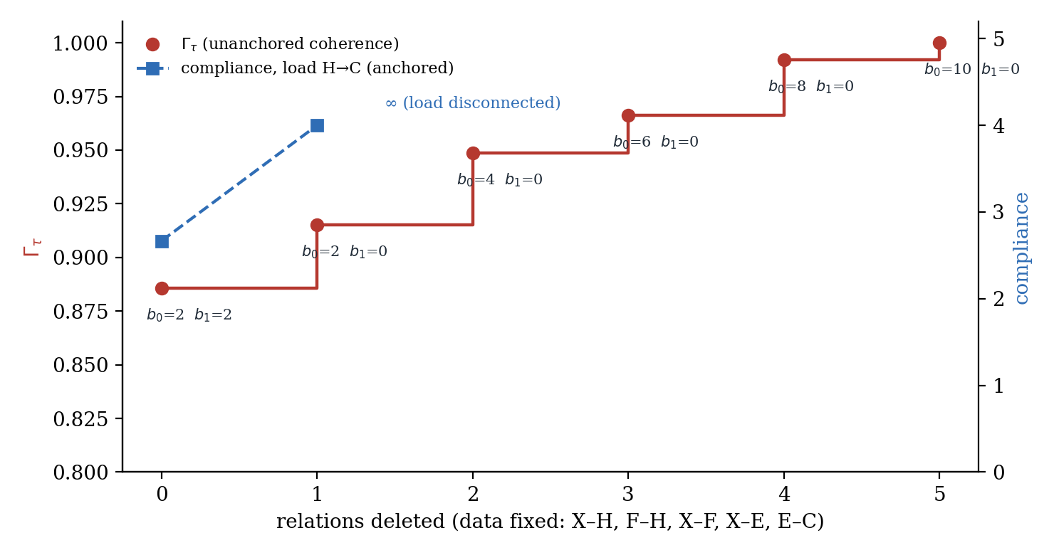
Computed (institutional sheaf, $\tau=0.5$ fixed). Edges were deleted in the order X–H, F–H, X–F, X–E, E–C.
| Edges deleted | $\Gamma_{\tau}$ | $b_0$ | $b_1$ | Compliance, load H→C |
|---|---|---|---|---|
| 0 | 0.886 | 2 | 2 | 2.667 |
| 1 (X–H) | 0.915 | 2 | 0 | 4.000 |
| 2 (F–H) | 0.949 | 4 | 0 | ∞ |
| 3 (X–F) | 0.966 | 6 | 0 | ∞ |
| 4 (X–E) | 0.992 | 8 | 0 | ∞ |
| 5 (E–C) | 1.000 | 10 | 0 | ∞ |
The first deletion (X–H) lowered $b_1$ from 2 to 0. Every later deletion raised $b_0$. Measured coherence rose monotonically to 1 with no datum changed [E].
19.3 Readings
The theorem has four readings.
- Coherence by excision is always available. Any system can reach $\Gamma=1$ by deleting its relations. This is the formal reason the optimisation axiom N1 is a norm: measurement alone cannot forbid the efficient route to coherence. N1 forbids it because excision reduces structural diversity [D].
- Atomisation is perfect coherence. With every relation deleted, every individual is trivially consistent with itself and $b_0$ is maximal. This is the sheaf form of the atomised mass in Arendt’s account of totalitarian rule (Arendt 1951), read in The Totalitarian Sheaf (DRK-125) [D].
- Excision kills the invariant. By (iv), every deleted relation removes held difference ($b_1$ falls) or splits the system ($b_0$ rises). The Burnt Section (DRK-158) distinguishes “$H^1\to0$ via gluing” from “$H^1\to0$ via excision of stalks”. Theorem 19.2 makes the distinction computable [D].
- Deleting measurement converts fault into fate. By (iii), ceasing to measure the interior of a loop turns a local, attributable circulation into a systemic, unattributable class. Diffusion of responsibility has this exact form: the loss is unchanged, but no face can be held for it [D].
19.4 The admissibility rule
Definition 19.3 (Excision report). Every reported coherence change between $(X,\mathcal F)$ and $(X',\mathcal F')$ carries the excision vector $$\chi_{\text{exc}}=\big(\Delta\dim C^0,\ \Delta\dim C^1,\ \Delta\dim C^2;\ \Delta E;\ \Delta b_0,\ \Delta b_1\big),$$ together with the coherence recomputed on the common base [D].
Corollary 19.5 (Inversion filter, computable). A coherence gain is classified by recomputing it on the original base:
- if it vanishes on the original base, it was produced by excision and is classified as a manufactured void (KO V.7);
- if it persists, it was produced by gluing.
Proof. By Theorem 19.2(i), the remaining gain on a fixed base is attributable to changes of data or maps, not to the base. ∎ [E/D]
19.5 The anchored dual: compliance and Rayleigh monotonicity
Theorem 19.2 shows that an unanchored coherence measure rewards excision. Its dual shows that an anchored measure punishes it.
Proposition 19.6 (Rayleigh monotonicity; compliance). Let $f\in C^0$ be a declared load, and let $\varepsilon>0$. Define the compliance $$c_\varepsilon(f):=\big\langle f,(L+\varepsilon I)^{-1}f\big\rangle .$$ Then $c_\varepsilon(f)$ is non-decreasing under relation excision and non-increasing under adding relations.
As $\varepsilon\to0$ with $f\perp H^0$, $c_\varepsilon(f)\to\langle f,L^+f\rangle$. For the constant scalar sheaf and $f=\mathbf e_u-\mathbf e_v$, this limit is the effective resistance between $u$ and $v$. If excision disconnects the support of $f$, the compliance diverges [E].
Proof. Excision gives $L'\preceq L$, hence $L'+\varepsilon I\preceq L+\varepsilon I$. Inversion reverses the order. The effective-resistance identity is standard (Doyle & Snell 1984). ∎ [E]
For the constant scalar sheaf this is Rayleigh’s monotonicity law: cutting wires never lowers resistance (Doyle & Snell 1984) [E].
Compliance has a second meaning that ties it to measurement. When node values are estimated from noisy relative measurements, the variance of the estimated difference between $u$ and $v$ is proportional to the effective resistance between them (Barooah & Hespanha 2008). Excision therefore raises not only the cost of carrying a load but also the uncertainty with which the remaining system can know its own differences. Unanchored coherence goes up while the ability to verify it goes down [E/D].
Computed (institutional sheaf, unit load between H and C). The compliance is 2.667 on the full complex, 4.000 after deleting X–H, and infinite once F–H is also deleted and H is disconnected. Over the same deletions, the unanchored $\Gamma_\tau$ rose from 0.886 toward 1 (§19.2) [E].
Topology optimisation. Structural topology optimisation removes material deliberately. It minimises compliance $f^\top K(\varrho)^{-1}f$ subject to $K(\varrho)u=f$ and a volume bound $\int\varrho\le V^\ast$ (Bendsøe & Sigmund 2003). The Compartmentalized Manifold (DRK-161) applies this formulation to institutional design [E/D].
Engineering has long had the answer to totalisation:
- Excision is permitted only under a load. The load $f$ is an anchor, and removing a member that carries load is penalised by the objective itself.
- Without a load, the optimum is to remove everything, which is Theorem 19.2(i).
Corollary 19.7 (Anchored admissibility). A coherence intervention is admissible only if two conditions hold:
- it passes Corollary 19.5 (the gain persists on the original base);
- it does not raise the compliance $c_\varepsilon(f)$ for the declared loads $f$, i.e. for the demands the system exists to carry.
The first condition forbids hidden excision. The second forbids visible excision that sheds load-bearing relations [D].
Proof of consistency. By Proposition 19.6, any relation excision weakly raises compliance, and it raises it strictly when the deleted relation carries part of the load. ∎ [E]
19.6 The rule applies to Draken
The corpus’s structural score, Watertightness $W$, is computed over the fixed set of published posts (Chapter 23). Raising $W$ by unpublishing poorly referenced posts would be excision under Definition 19.1 [D].
v5.0 therefore lists the disposition of every DRK post (Appendix E). Posts excluded from the monograph are excluded from its argument, not from the corpus. The anti-totalisation principle applies to Draken itself [D].
Part VI — Programme, Computation, Falsification
20 The Empirical Programme
Each item below names a domain, the declared sheaf, the Draken quantity, and the outcome that would count against it. Items are ordered by readiness [D].
20.1 Varanid ritualised combat (ready; existing data)
Domain. Monitor lizards resolve contests through a ritualised sequence: display, encompassing, clinch, catch and a final dominance phase, labelled subpressive in the approved KO definition of the Clinch (DRK-108). In this sequence, physical grappling tests the claims made by display (Horn, Gaulke & Böhme 1994; Earley, Attum & Eason 2002) [S]. Source check pending: DRK-108 attributes the five-phase description to “Horn, Gauldie, and King (1994)”, while v4.4 cites Horn, Gaulke & Böhme (1994). Neither could be machine-verified, and the phase labels must be checked against the primary source before P8 is run [D].
Sheaf. Vertices are phases, and stalks are the measured state per phase. The restriction maps are parameterised by body mass (Frýdlová et al. 2016) and musculoskeletal scaling (Dick & Clemente 2016). The clinch is the anchor that zeroes the bluff kernel (Section 16.3) [D].
Test (P8). Compute $\Gamma_{\tau}$ at fixed base for the sheaf induced by each competing contest model:
- sequential assessment;
- energetic war of attrition;
- cumulative assessment (Enquist & Leimar 1983).
The model with the highest coherence should best predict transition probabilities and outcomes across species. Falsifier: coherence ranks models no better than a random-map null [H].
20.2 Representational drift (ready; public data)
Domain. Neural codes for stable tasks change over days to weeks while behaviour remains stable (Driscoll et al. 2017; Schoonover et al. 2021). Proposed explanations include self-healing codes and drift confined to null coding spaces (Rule & O’Leary 2022; Rule et al. 2020) [S].
Hypothesis H20.1 (Drift as gauge). Behaviourally silent drift is a stalk-wise orthogonal transformation with co-transforming readout maps. By Proposition 5.5(iii) such a transformation leaves every coherence measure invariant (Representational Drift as Sheaf-Theoretic Coherence, DRK-146) [H].
Test (P11). Decompose day-to-day changes of population vectors into a gauge part (the best orthogonal alignment, by Procrustes) and a residual. Prediction: behavioural decoding loss is explained by the residual, not by total drift. Falsifier: loss tracks total drift equally well [H].
20.3 Morphogenesis and regeneration (protocol published)
Domain. Bioelectric patterns act as an instructive layer between gene regulation and anatomy (Levin & Martyniuk 2018). Neural cellular automata learn to grow and regenerate target patterns (Mordvintsev et al. 2020) [S].
Sheaf. The Stalking Cell (DRK-167) proposes the restriction-map chain $$\text{DNA}\xrightarrow{\rho_1}\text{regulatory pathway}\xrightarrow{\rho_2}\text{bioelectric field}\xrightarrow{\rho_3}\text{tissue}\xrightarrow{\rho_4}\text{form}.$$ The Khrug Engineering protocol KE-NCA-001 specifies a sheaf over the cell lattice of a neural cellular automaton, with cell states as stalks [D].
Test (P12). After damage, the cell-state sheaf’s $\Gamma_{\tau}$ and spectral gap $\lambda_1^+$ recover before morphological error does. Falsifier: coherence recovery lags or merely tracks morphological recovery [H].
20.4 Inter-brain carrier and cargo (requires new data)
Test (P10). In hyperscanning, measure two quantities (The Carrier and the Cargo, DRK-189, §8):
- carrier coherence, as phase-locking value or $r^2$;
- cargo coherence, as $\Gamma_\tau$ of a belief sheaf estimated by representational similarity analysis (Kriegeskorte et al. 2008).
Prediction: the two dissociate across conditions (H13.1). Falsifier: they are interchangeable across all conditions [H].
20.5 Early warning of fragmentation (ready; network panel data)
Test (P9). In longitudinal interaction networks (organisations, online communities, alliances), track the projection of the data onto the slowest nonzero Laplacian mode.
Prediction: the variance and lag-1 autocorrelation of that projection rise before $b_0$ increases (Proposition 15.4; Scheffer et al. 2009). Falsifier: no rise relative to matched non-fragmenting periods [H].
20.6 Institutional and ecological diagnostics (v4.4 programme, sharpened)
Predictions P1–P7 of v4.4 are retained with v5.0 instruments [H]:
- the bounded companion $\bar\psi$ for Ψ;
- the outstanding balance $B_K$ and the measurable $K_\Gamma$ for debt;
- $\alpha^\ast$ for abstraction depth;
- $\Gamma_\tau$ at fixed base, with declared reference, noise correction and excision report, for coherence.
For ecological networks (P5), the null model is degree-preserving rewiring of the trophic complex. Γ must beat the null to count [D].
21 Computation
21.1 Pipeline
- Declare the complex $X$ (cells and orientations), stalks with inner products, restriction maps (estimated, with residuals), the reference $x_{\text{ref}}$, the stiffness τ (fixed on the reference base), and the coefficient field (Axioms A2, A4).
- Assemble $\delta^0,\delta^1$ as sparse block matrices.
- Vertex coherence. Solve $(I+\tau L)y=x$ by conjugate gradients. Then $\Gamma_\tau=\langle x,y\rangle/\|x\|^2$. No eigendecomposition is needed.
- Relational decomposition.
- Solve $Lx^\star=\delta^{0\top}\omega$ (minimum-norm least squares) for the gradient part.
- Solve $\Delta^2y=\delta^1\omega$ for the curl part.
- The harmonic part is the remainder.
- Report $E_{\text{grad}},E_{\text{harm}},E_{\text{curl}}$, and test $E_{\text{harm}}$ against the $\chi^2_{b_1}$ floor (Proposition 18.1).
- Invariants. Compute $b_0$, $b_1$ by rank (exact rational or $\mathbb F_2$ elimination for small or code-like complexes). Compute $\lambda_1^+$ and $s_1$ by Lanczos with shift-invert.
- Estimation. Apply the noise correction (Proposition 5.10) and sensitivity analysis (Proposition 5.9).
- Time series. Compute ratchet integrals by quadrature, the outstanding balance against recorded discharges, and early-warning statistics (Proposition 15.4).
- Comparisons. Recompute on the common base and attach the excision report (Definition 19.3).
[E/D]
21.2 Complexity
Write $n=\dim C^0$ and $\operatorname{nnz}(L)=O(|E|\,d_{\max}^2)$.
| Step | Cost | Note |
|---|---|---|
| Assemble $L$ | $O(\lvert E\rvert\,d_{\max}^3)$ | Block products $\rho^\top\rho$ |
| Matrix–vector product | $O(\operatorname{nnz}(L))$ | Corrects v4.4’s $O(n\lvert E\rvert)$ |
| $\Gamma_\tau$ by CG | $O\big(\operatorname{nnz}(L)\sqrt{1+\tau\lambda_{\max}}\,\log(1/\epsilon)\big)$ | Well conditioned; independent of the spectral gap |
| $\Gamma_0$, $x^\star$ | Governed by $\lambda_1^+$ (ill-conditioned near fragmentation) | Prefer $\Gamma_\tau$ |
| $\lambda_1^+$, $\lambda_{\max}$, $s_1$ | $O(k\cdot\operatorname{nnz})$ per Lanczos sweep | |
| $b_1$ exact | Sparse rank; $O(n^3)$ dense worst case | $\mathbb F_2$ elimination for codes |
The conditioning of the resolvent system is bounded by $1+\tau\lambda_{\max}$ regardless of how small the spectral gap becomes. This is a practical reason, beyond Proposition 5.6, to prefer $\Gamma_\tau$ as the canonical measure [E].
21.3 Instruments
- The Sheaf Analyzer (The Sheaf Analyzer, DRK-132) already computes coboundaries of text-derived sheaves. v5.0 specifies the additions:
- $\Gamma_\tau$ with declared τ and reference;
- the three-part decomposition for relational extractions;
- $b_1$ and $s_1$;
- the noise floor of Proposition 18.1.
- The KnowledgeObject schema (KnowledgeObject Schema v2, DRK-101) is the corpus’s typed memory, and the KO registry (Appendix B) is its current state.
- The reproducibility script of Appendix F implements steps 2–6 for the worked examples.
[D]
22 Falsification
22.1 What can and cannot be falsified
The monograph contains three kinds of statement, and they fail in different ways [D]:
- Theorems and propositions (Chapters 2–5, 9, 12, 15, 18, 19). These are checked, not tested. They fail only by an error in the proof, and each one numbered in a worked example is also checked numerically by the script. A reader who finds an error falsifies the proposition and every reading built on it.
- Bridges (Chapter 10 ledger). An exact bridge fails if the identification is shown not to hold. An analogy cannot fail as evidence because it is never used as evidence.
- Empirical hypotheses and predictions, listed below.
The protocol is the DRK-131 falsification protocol (approved KO, defined in The Braided Substrate, DRK-143, §7). It requires no fabricated citations, verified paraphrase, an explicit falsification subsection and a three-question review [D].
22.2 Predictions
| # | Prediction | Instrument | Falsifier | Status |
|---|---|---|---|---|
| P1 | Higher $\bar\psi$ precedes strategic failure | Ψ pipeline (Ch. 6) | No association in longitudinal panel | Untested (v4.4) |
| P1′ | (Γ, $\bar\psi$) is not inversely related; the kayfabe quadrant is populated | Γ_τ, $\bar\psi$ | Joint distribution concentrated on the anti-diagonal | New; untested |
| P2 | Larger outstanding debt $B_K$ precedes larger corrections | $K$, $P_K$, $K_\Gamma$ | Correction size independent of $B_K$ | Partially tested retrospectively (v4.4) |
| P3 | Larger $\alpha^\ast$ precedes slower correction | $\alpha^\ast$ (Ch. 8) | No association | Untested |
| P4 | Restriction-map repair raises $\Gamma_\tau$ on a fixed base | Γ_τ + excision report | No rise, or rise only by excision | Untested |
| P5 | Trophic $\Gamma_\tau$ tracks ecosystem health | Γ_τ vs rewired null | No better than null | Testable now |
| P6 | Removal of enforcing institutions raises $\bar\psi$ | $\bar\psi$ | No change | Retrospectively testable |
| P7 | Attention-economy $\alpha^\ast$ predicts population-level $\bar\psi$ | $\alpha^\ast$, survey Ψ | No association | Testable now |
| P8 | Contest-model coherence predicts varanid outcomes | Section 20.1 | No better than random-map null | Testable now |
| P9 | Rising variance and autocorrelation of the slow mode precede fragmentation | Prop. 15.4 | No rise vs matched controls | New; testable now |
| P10 | Carrier and cargo coherence dissociate | Section 20.4 | Interchangeable across conditions | New; requires data |
| P11 | Behavioural loss tracks the non-gauge part of drift | Section 20.2 | Equal fit for total drift | New; testable now |
| P12 | Coherence recovers before form in regeneration | Section 20.3 | Lag or mere tracking | New; protocol published |
| P13 | Claimed-minus-measured coherence ($K_\Gamma$) predicts correction size beyond $E_{\text{obs}}$ | H7.1 | No incremental prediction | New |
| P14 | Coherence gains that vanish on the original base (Cor. 19.5) precede larger corrections than gains that persist | Excision report | No difference | New |
| P15 | Interventions that raise Γ while raising load compliance (Cor. 19.7) precede service failures under those loads | $\Gamma_\tau$, $c_\varepsilon(f)$ | No association | New |
| P16 | In food webs, deviation of measured transfer profiles from the Lindeman section predicts instability indices | Prop. 16.3 | No association beyond biomass alone | New; testable now |
22.3 Framework-level falsifiers
The framework as a diagnostic programme fails in any of the following cases [D]:
- F-A. Across at least three domains, $\Gamma_\tau$ at fixed base predicts its target (P4, P5, P8) no better than its matched null.
- F-B. In domains where a Draken reading claims a structural obstruction, $E_{\text{harm}}$ does not exceed its noise floor (Proposition 18.1).
- F-C. The debt measures (P2, P13, P14) add nothing to prediction beyond contemporaneous coherence.
Scope limit. The proofs establish that the measures are well defined, computable and correctly invariant. They do not establish that the measures matter for any particular system. That is what F-A to F-C test [D].
23 Governance and Self-Audit
23.1 Guarding the framework against its own use
v4.4 translated the V-axioms into system requirements, and they are retained [D]:
| Axiom | Requirement |
|---|---|
| V.1 | Log every restriction-map modification with author and time |
| V.2 | Compute the system’s own Ψ on its outputs |
| V.4 | Alert on rising Ψ in its own analyses |
| V.7 | Apply the framework’s criteria to its own claims before publication |
v5.0 adds two requirements [D]:
- Every coherence claim carries the reporting standard 5.7a and, for comparisons, the excision report (Definition 19.3).
- No reported number is hand-kept. Every statistic is computed from data at build or by script.
23.2 Watertightness is not coherence
The corpus’s structural score is Watertightness W v2 (released 2026-10-01; docs/W-VERSIONS.md in the site repository): $$W=\big(c_7^{3}\,c_1\,c_2\,c_3\,c_4\,c_6\big)^{1/8},\qquad W_{\text{post}}=\big(c_7^{3}\,c_1\,c_6\big)^{1/5}.$$ The components are:
- $c_1$, reference integrity;
- $c_2$, definition coverage;
- $c_3$, KO closure;
- $c_4$, KO reuse;
- $c_6$, citation connectivity;
- $c_7$, claim paragraphs carrying a reference (weight 3).
Component $c_5$ (falsification block) was removed in v2 and is not reused [E].
On 2026-10-02 the corpus scored W = 0.745. Its components were $c_1$ = 0.986, $c_2$ = 0.938, $c_3$ = 1, $c_4$ = 0.906, $c_6$ = 1 and $c_7$ = 0.483 (668 of 1,382 claim paragraphs referenced). $c_7$ is binding [E].
W measures the structure of the record (references, definitions and their reuse, connectivity), not the truth of its claims. It is never labelled Γ. Changing its patterns or weights after seeing results requires a new version [D].
23.3 Self-audit: v4.4 against v5.0
| Measure | v4.4 | v5.0 |
|---|---|---|
| Corpus covered | DRK-101–121 (14 posts that exist; 16 claimed) | All 86 posts dispositioned; 55 used in the argument (Appendix E) |
| Citations of nonexistent DRK numbers | 2 (DRK-109, DRK-122) | 0 |
| Errors found (arithmetic, logical, bibliographic) | 13 (Appendix D) | 0 known; every example recomputed by script |
| Numbered results with proof | 0 (one “derivation” sketch) | 45, each with proof or standard citation: 23 standard, 13 elementary, 9 original (Appendix G) |
| Worked examples computed by code | 0 | 8 examples + 7 propositions verified numerically |
| Figures generated from code | 0 | 6 of 6 |
| Inconsistent definitions in corpus | Not addressed | 13 forks settled (Appendix C) |
| Coherence measure range | Unbounded below (“Γ < 0”) | $(0,1]$, with bounds, invariances, monotonicity, estimator |
| Knowledge Objects integrated | 14 of today’s 32 terms present | 32 of 32 in the glossary; 27 used in the argument (Appendix B) |
| Bridge claims graded | No | 28 graded; 7 corpus claims excluded with reasons |
| Epistemic markers | Three-level | Five-tag ledger of the post standard |
| Claim paragraphs tagged | Section-level markers only | 220 of 220 claim paragraphs; 37 result statements tagged at their proofs (audit script, Appendix F) |
The v5.0 column is generated from the source by the audit step of the build script, apart from the counts of forks and bridges, which are enumerated in Appendix C and Chapter 10 [E].
24 Conclusion
What is proved. Model a multi-scale system as a cellular sheaf on a finite 2-complex. Then:
- its relational data split uniquely into a part that local re-gauging removes, a topological part (ϰ) and a curvature part;
- local relaxation removes exactly the first and stops exactly at the other two;
- coherence of local states is measured by a resolvent quantity with a repair-cost meaning, sharp spectral bounds, the correct invariances, and a monotonicity under adding and deleting relations;
- that monotonicity makes totalisation, coherence bought by deleting relations, always available. A norm, not a measurement, must forbid it.
- the same excision raises compliance under any declared load (Rayleigh monotonicity), so anchored measures detect what unanchored ones reward;
- obstructions reached by lifting across a cut and by integrating relational data are the same class (Proposition 3.11);
- the repair behind Γ is Bayesian denoising, which ties coherence to Gaussian Markov random fields and to score-based generation (Propositions 5.12, 15.5);
- trophic structure, input–output planning and iterated repair close onto the same linear algebra (Propositions 16.3–16.5).
[E/D]
What is computed. Every worked example, including corrected versions of v4.4’s two, is reproducible from a published script. Clock rings, U(1) rings, exchange complexes, toric codes, Kuramoto populations and signed triangles all instantiate the same three-part structure [E].
What is hypothesised. The same structure, applied to measured data from minds, groups, institutions and ecosystems, separates repairable from irreducible disagreement. Debt accrued by denying the irreducible part predicts the size of later corrections [H].
What must be tested. Predictions P1–P16 and framework falsifiers F-A to F-C. The most immediately executable are P5, P8, P9 and P11, on existing data [D].
Draken adds layers of explanation. It does not decide which global section is true, because no coherence measure can (Proposition 5.8). That decision belongs to the anchors: to contact with what lies outside the system’s own sections. The Clinch awaits [D].
Appendices
Appendix A — Notation Registry
Each symbol below has exactly one meaning in v5.0. The right-hand column records corpus usages that were renamed to remove collisions.
| Symbol | Meaning | Defined | Collisions resolved |
|---|---|---|---|
| $X$; $V,E,F$ | Regular 2-complex; vertices, edges, faces | Def. 2.1 | |
| $\mathcal F$, $\mathcal F(\sigma)$ | Cellular sheaf; stalk on cell σ | Def. 2.2 | |
| $\rho_{\sigma\tau}=\mathcal F_{\sigma\trianglelefteq\tau}$ | Restriction map (KO ρ) | Def. 2.2 | Density → $\varrho$; density matrix → $\hat\rho$; soundness → $\rho_s$; spectral radius → $\operatorname{sr}$; productile rank (DRK-141) → $P_r$ |
| $C^k$, $\delta^k$ | Cochains, coboundary | Def. 2.4 | |
| $H^k$, $b_k$ | Cohomology, Betti numbers | Def. 2.6 | |
| $L_{\mathcal F}=\Delta^0$ | Sheaf Laplacian (KO) | Def. 3.0 | |
| $\Delta^1,\Delta^2$ | Hodge Laplacians | Def. 3.0 | |
| $\Pi_{\text{grad}},\Pi_{\text{harm}},\Pi_{\text{curl}}$ | Hodge projectors on $C^1$ | §3.2 | |
| $E(x)$ | Disagreement energy $\|\delta^0x\|^2$ | §3.1 | |
| $E_{\text{grad}},E_{\text{harm}},E_{\text{curl}},E_{\text{obs}}$ | Component and obstruction energies | Prop. 3.2, Def. 3.2a | |
| $\mathcal R=\delta^1\omega$ | Curvature of relational data | Prop. 3.4 | |
| $\varkappa(\omega)$ | Draken invariant $[\Pi_{\text{harm}}\omega]$ (KO) | Def. 3.5 | |
| $\Phi_\gamma$ | Holonomy (period) on cycle γ | Prop. 3.6, 4.1 | DRK-171 “Θ” → $\Phi_\gamma$ |
| $\Gamma_\tau$, $\tau^\ast$ | Resolvent coherence (KO Γ); default stiffness | Def. 5.1 | v4.4 $1-R$, DRK-185 $1-\sqrt R$ retired |
| $\Gamma_0,\Gamma_R,\Gamma^1,\Gamma_{\text{top}}$ | Global share; spectral bound; integrability share; structural index | §5.7 | |
| $R(x)$ | Rayleigh quotient $E/\|x\|^2$ | Prop. 5.3 | |
| $\lambda_1^+$, $\lambda_{\max}$ | Spectral gap; top eigenvalue of $L$ | Prop. 5.4 | |
| $\mathcal U$ | Undetectable subspace $H^0\cap\ker A$ | Prop. 5.8 | |
| $\Psi$, $\bar\psi$ | Narrative self-reference (odds, KO); bounded share | §6.1 | DRK-176 basin “Ψ” → $\beta_{\text{self}}$; quantum Ψ → $\lvert\psi\rangle$ |
| $\sigma(t)$ | Synchronicity density (KO) | §6.4 | |
| $\mathcal D[f,w]$ | Ratchet functional | Def. 7.1 | |
| $K(t)$, $B_K$, $P_K$, $K_\Gamma$ | Coherence debt (KO); balance; discharge; measurable instance | §7.1–7.3 | DRK-130, DRK-141, DRK-176 “K” → $I(t)$, $G(t)$, $C(t)$ |
| $\Theta(t)$ | Trophic debt (KO) | §7.1 | |
| $D_k$ | Stage deficit (earth engine) | §7.1 | |
| $\mathcal V$, $\dot{\mathcal V}_{\text{exo}}$ | Variety; exogenous variety change (care, KO) | §7.5 | |
| $\alpha$, $\alpha^\ast$ | Abstraction depth (KO); path-minimal form | Def. 8.1–8.2 | |
| $\mathfrak W=(b_1,d,\rho_s)$, $s_1$ | Warded triple (KO); spectral soundness | §9.2 | |
| $S_{\text{sys}}$, $H$ | Disorder; structural diversity (Norm N1) | §2.1 | |
| $c,V,\theta$ | Certainty, value, threshold (conviction gate, KO) | §17.2 | |
| $\chi_{\text{exc}}$ | Excision report | Def. 19.3 | |
| $\mathcal K\to\mathcal E\to\mathcal Q$ | Short exact sequence of sheaves | Def. 3.9 | Calligraphic; distinct from debt $K(t)$ |
| $\partial$, $\omega_q$ | Connecting map; lifting datum | Thm. 3.10, Prop. 3.11 | |
| $\sigma$; $\sigma(t)$; $\sigma(\mathcal F)$, $\sigma_\varepsilon$ | Noise standard deviation; synchronicity density (KO); agreement fractions | Props. 5.10, 15.4; §6.4; Prop. 5.11 | Distinguished by argument; the v4.4 symbol $\sigma_{\text{self}}$ is replaced by $\bar\psi$ and the count $n_{\text{self}}$ |
| $R_\tau$, $P$ | Repair (resolvent); projection onto $H^0$ | Prop. 5.12, 16.5 | |
| $\mathsf e$, $\mathsf b$ | Trophic transfer efficiency; biomagnification factor | Prop. 16.3 | Not the noise ε or the monad unit |
| $\mathsf D$, TL | Diet matrix; trophic levels | Prop. 16.4 | |
| $(\mathbb T,\eta_{\mathbb T},\mu_{\mathbb T})$ | Monad | §16.6 | Subscripted to avoid the noise symbol |
| $c_\varepsilon(f)$ | Compliance under load $f$ | Prop. 19.6 |
Appendix B — Glossary of Knowledge Objects
All 32 Knowledge Objects in the registry (data/ko.json, generated 2026-10-02) are approved. Each definition below is quoted verbatim from its defining post, in the post’s language. Where a definition ends in a colon, the defining formula follows in the source. The last field gives where the KO is used in this monograph. Registry gap: anti-totalisation appears in 37 posts but has no KO. Chapter 19 supplies its formal content, and a defining post is needed before it can be registered.
Γ — sheaf convergence — aliases: Γ, \Gamma, Gamma, sheaf convergence, sheaf coherence, kärvskonvergens
The sheaf convergence measure Γ (gamma) tracks the inverse: how well local sections glue into a globally consistent picture.
Defined in The Kaiju Manifesto: Building the Anti-Memetic Monster (DRK-105, The 18-Layer Architecture). Status: approved. Used in v5.0: Ch. 5.
Ψ — narrative self-reference ratio — aliases: Ψ, \Psi, Psi, narrative self-reference ratio, narrative self-reference, psykosmetrik
Ψ (psi) is the psychosis metric — the ratio of narrative self-reference to reality-contact.
Defined in The Kaiju Manifesto: Building the Anti-Memetic Monster (DRK-105, The 18-Layer Architecture). Status: approved. Used in v5.0: Ch. 6.
K(t) — coherence debt — aliases: K(t), coherence debt, koherensskuld
*This article introduces the coherence debt function K(t) — the temporal integral of excess Ψ above viable threshold — and argues that what spiritual traditions have called karma, what systems theorists have called fragility, and what the Draken framework diagnoses as civilizational Ψ-degradation are structurally identical phenomena: the accumulated cost of running a generative model that refuses correction.
Defined in The Coherence Debt: Karma as Thermodynamic Integral (DRK-121, opening). Status: approved. Used in v5.0: Ch. 7.
ϰ — Draken invariant — aliases: ϰ, \varkappa, Draken invariant, invariant of Draken
The invariant is cohomological: discrete, preserved under the sheaf analogue of ambient isotopy.
Defined in The Invariant (DRK-175, §4 — The invariant of Draken.). Status: approved. Used in v5.0: Ch. 3, 9.
ρ — restriction map — aliases: ρ, restriction map, restriction morphism, restriktionsavbildning
I kärv-teori beskriver restriktionsavbildningen ρ_U,V : F(U) → F(V) hur information över ett stort område (U) begränsas till ett mindre delområde (V ⊆ U).
Defined in Drakens Ordlista: Kärnbegrepp för nybörjare (DRK-117, Restriktionsavbildning (Restriction Map)). Status: approved. Used in v5.0: Ch. 2.
H¹ — cohomological obstruction — aliases: H¹, H^1, cohomological obstruction, obstruction class, kohomologisk obstruktion
Tekniskt: ett icke-trivialt element i H¹(X, F) — den första kohomologigruppen av kärven F över rummet X.
Defined in Drakens Ordlista: Kärnbegrepp för nybörjare (DRK-117, Kohomologisk obstruktion). Status: approved. Used in v5.0: Ch. 2–3.
**Care operator V̇_exo = 0** — aliases: care operator, V̇_exo, \dot{V}_{exo}, \dot{\mathcal V}_{exo}, omsorgsoperatorn
The care operator is the condition $\dot{\mathcal V}_{exo}=0$: the non-destruction of exogenous variety — the commitment not to annihilate the otherness of the thing you are bound to.
Defined in The Bridge and the Burn (DRK-162, Frankenstein: assembly without the seam). Status: approved. Used in v5.0: Ch. 2, 7.
Θ — trophic debt — aliases: Θ(t), \Theta(t), trophic debt, trofisk skuld
Define trophic debt as the accumulated violation of care:
Defined in Ouroboros Debt (DRK-176, §4 — Trophic debt: the bill for closing the loop). Status: approved. Used in v5.0: Ch. 7.
Optimization axiom — aliases: optimization axiom, optimeringsaxiomet, min S_sys
“Minska oordningen i systemet — men inte genom att förenkla bort komplexiteten.”
Defined in Drakens Ordlista: Kärnbegrepp för nybörjare (DRK-117, Optimeringsaxiomet). Status: approved. Used in v5.0: Ch. 2, 19.
Manufactured void — aliases: manufactured void, tillverkad tomhet, narrative void engineering
“När maktstrukturer medvetet skapar informationshål för att styra vilka berättelser som kan bildas.”
Defined in Drakens Ordlista: Kärnbegrepp för nybörjare (DRK-117, Tillverkad Tomhet (Manufactured Void / DRK-110)). Status: approved. Used in v5.0: Ch. 18–19.
Cavity_AI — cavity resonator — aliases: Cavity_AI, kavitetsresonator, cavity resonator
“En strukturerande tomhet som formar allt som passerar genom den.”
Defined in Drakens Ordlista: Kärnbegrepp för nybörjare (DRK-117, Cavity_AI — Kavitetsresonatorn). Status: approved. Used in v5.0: Glossary only (companion volume).
Inversion filter (V.7) — aliases: Inversion Filter, inversionsfilter, V.7
Det viktigaste diagnostiska verktyget: om en struktur hävdar att den erbjuder global koherens men kräver informationsundertryckning vid sina gränser, är den en tillverkad tomhet — inte en genuin gräns.
Defined in Drakens Ordlista: Kärnbegrepp för nybörjare (DRK-117, V-axiomen — Drakens värdeaxiom). Status: approved. Used in v5.0: Ch. 18–19.
α — abstraction depth — aliases: abstraction depth, abstraktionsdjup
We define abstraction depth as the number of representational layers between a claim to power and the capacity that underlies it:
Defined in Abstraction Depth: Why Your Boss Doesn’t Have to Wrestle You (DRK-108, II. The Primate Who Learned to Abstract). Status: approved. Used in v5.0: Ch. 8.
Clinch — aliases: clinch, klinch
Horn, Gauldie, and King (1994) described five distinct phases: Display, where the animals inflate their bodies laterally, maximizing apparent size; Encompassing, where they circle each other, assessing geometry; Clinch, where they rear up on hind legs and lock forelimbs in bipedal wrestling; Catch, where one animal attempts to topple the other using what researchers have described as judo-like throws; and Subpressive, where the victor mounts the defeated animal in a dominance display.
Defined in Abstraction Depth: Why Your Boss Doesn’t Have to Wrestle You (DRK-108, I. A Life Measured in Grapples). Status: approved. Used in v5.0: Ch. 16, 20.
Kayfabe — aliases: kayfabe, kayfabe trap
When the framework’s diagnostic output flags Ψ → 1 with restriction maps collapsing — kayfabe, in the working vocabulary — what it has detected is a configuration that has become locally coherent at the cost of severing its accountability to the larger system.
Defined in The Protocol and the Predator: On Asymmetric Power Without Extraction (DRK-133, I. Two Asymmetries). Status: approved. Used in v5.0: Ch. 6, 18.
Survivable glitch — aliases: survivable glitch, ∇_s, \nabla_s
A failure mode whose information content survives the failure event, gets fed back into the design layer, and improves the protocol for the next iteration.
Defined in The Survivable Glitch: Lacan’s Middle Period, the Simulator, the Haveriutredning, and Why I Named the Framework Draken (DRK-138, III. The Survivable Glitch: Where Engineering Anticipated Philosophy). Status: approved. Used in v5.0: Glossary only (companion volume).
Source laundering — aliases: laundering operator, source laundering, laundering, laundered, launder
It is a substitution at the stalk — he replaces $\mathcal{F}_s =$ “leader of warriors” with a forged value $\mathcal{F}_s' =$ “head of the dragon (because: comet),” and then forces every downstream section to glue to the forgery:
Defined in The Pendragon Source (DRK-165, II. The laundered name (Geoffrey’s pen)). Status: approved. Used in v5.0: Ch. 18.
Carrier — aliases: carrier, bärare
The first is coordination: the degree to which the group’s neural activity is temporally aligned, phase-locked, beating together.
Defined in The Carrier and the Cargo: Phase Synchrony, Representational Content, and the Cohomology of a Shared Belief (DRK-189, 1. Two layers, never to be conflated). Status: approved. Used in v5.0: Ch. 13.
Cargo — aliases: cargo
The second is representational alignment: the degree to which the group now holds the same belief, the same vector in some semantic space.
Defined in The Carrier and the Cargo: Phase Synchrony, Representational Content, and the Cohomology of a Shared Belief (DRK-189, 1. Two layers, never to be conflated). Status: approved. Used in v5.0: Ch. 13.
Chaxu geju (差序格局) — aliases: chaxu geju, 差序格局, differentiell associationsmod
Fei Xiaotongs begrepp från 1947: kinesisk social struktur organiseras som koncentriska ringar runt individen — familj närmast, sedan släkt, sedan grannar, sedan samhälle — med moralisk förpliktelse som avtar med avstånd.
Defined in Drakens Ordlista: Kärnbegrepp för nybörjare (DRK-117, Chaxu geju (差序格局) — Differentiell associationsmod). Status: approved. Used in v5.0: Glossary only (companion volume).
Sheaf Laplacian — aliases: sheaf Laplacian, \Delta_{\mathcal{F}}, L_F, L_{\mathcal{F}}, kärv-Laplacian
The sheaf Laplacian is $\Delta_{\mathcal{F}} = \delta^T \delta$, where $\delta$ is the coboundary operator measuring disagreement on edges.
Defined in The Operational Question in Positive Alignment (DRK-145, 1. Sheaf-theoretic machinery for cross-scale coherence). Status: approved. Used in v5.0: Ch. 3.
Global section — aliases: global section, global sections, globala sektioner, global sektion
A global section is an assignment $\{x_v \in \mathcal{F}(v)\}_{v \in V}$ such that $\rho_{u \to e}(x_u) = \rho_{v \to e}(x_v)$ for every edge $e = (u,v) \in E$.
Defined in The Operational Question in Positive Alignment (DRK-145, 1. Sheaf-theoretic machinery for cross-scale coherence). Status: approved. Used in v5.0: Ch. 2.
DRK-131 falsification protocol — aliases: DRK-131 protocol, DRK-131 publishing protocol, falsification protocol, Falsification (DRK-131), Falsifiering (DRK-131)
The DRK-131 protocol exists precisely to discipline this risk: no fabricated citations, verified paraphrases, explicit falsification subsection, three-questions review.
Defined in The Braided Substrate: Berry Curvature, Tensor Networks, and Why Topology Builds Draken (DRK-143, 7. Falsification). Status: approved. Used in v5.0: Ch. 22.
Keeper-function — aliases: keeper-function, keeper function, keeper-of-secrets, Generalizard
Four conditions are required of any node to instantiate this keeper-function:
Defined in The Generalizard: Keeper-Function, Mandate, and the Imperial Dragon (DRK-150, 2. The Four Structural Conditions for Keeping). Status: approved. Used in v5.0: Glossary only (companion volume).
σ(t) — synchronicity density — aliases: synchronicity density, σ(t)
Synchronicity density $\sigma(t)$ is the fraction of salient events at time $t$ that the observer reads as addressed to the self [D].
Defined in The Common Base: Dream Logic, Archetype, and the Coincidence That Needs No Channel (DRK-177, §8). Status: approved. Used in v5.0: Ch. 6.
𝔚 — warded invariant — aliases: warded invariant
$$\mathfrak W(\mathcal F) := \big(\, b_1,\ \ d,\ \ \rho \,\big)$$
Defined in The Warded Class: Quantum Codes as Sheaves, and What H¹ Protects (DRK-190, §8 Proposal: the warded invariant). Status: approved. Used in v5.0: Ch. 9.
Egregore — aliases: egregore, egregores, egregor
The Draken reading is that an egregore is a well-glued section whose stability no longer depends on any single stalk [D].
Defined in The Compressed Will: Sigils, Grimoires, Egregores and Curses as Operations on Symbolic Maps (DRK-191, §7 Egregores: sections that outlive their stalks). Status: approved. Used in v5.0: Ch. 6.
Stalk — aliases: stalk, stalks
The stalk of $\mathcal F$ at a point $x \in X$ is the direct limit $$\mathcal F_x \;=\; \varinjlim_{U \ni x} \mathcal F(U),$$ taken over all open neighbourhoods of $x$.
Defined in The Stal King: Stalking, the Eye on the Stalk, and the Germ at the Point (DRK-192, §2 Formal sketch: the stalk as limit of a pursuit (analogy, not derivation)). Status: approved. Used in v5.0: Ch. 2.
Stalking — aliases: stalking
Stalking (proposed corpus term): a pursuit that refines a nested family of neighbourhoods around a target while keeping its own estimates restriction-compatible and keeping its own contribution to the target’s observations at zero [D].
Defined in The Stal King: Stalking, the Eye on the Stalk, and the Germ at the Point (DRK-192, §2 Formal sketch: the stalk as limit of a pursuit (analogy, not derivation)). Status: approved. Used in v5.0: Glossary only (companion volume).
Earth engine — aliases: earth engine
The earth engine (proposed corpus term): the reading of the Earth system as a cascade of heat engines fired by the Sun, in which each stage compresses usable form from the stage above, burns it through a gate, and fails in one of a small number of engine fault modes [D].
Defined in The Earth Engine: A Sun-Fired Cascade, Minds as Charge, and the Failure Modes of a Planet (DRK-193, §3 Formal sketch: stocks, gates and debts (analogy, not derivation)). Status: approved. Used in v5.0: Ch. 16.
Conviction gate — aliases: conviction gate, conviction gates
The conviction gate (proposed corpus term) is this inequality: the point where a belief is allowed to command action, governed by certainty, by the value attached to the act, and by the threshold that others and one’s own norms impose [D].
Defined in The Conviction Gate: How a Pattern Becomes a Belief That Acts (DRK-194, §2 Formal sketch: precision and the gate (analogy, not derivation)). Status: approved. Used in v5.0: Ch. 17.
Gate capture — aliases: gate capture, captured gate
Gate capture (proposed corpus term): the condition in which the value of acting, the threshold for action, or the certainty of the belief is set by an agent other than the believer, so that the believer’s gate opens on someone else’s terms [D].
Defined in The Weaponised Conviction: Recruitment, Amplification, and the Self Turned Inward (DRK-195, §1 Gate capture). Status: approved. Used in v5.0: Ch. 17–18.
Appendix C — Decision Record: Forks Settled for v5.0
| # | Fork | Corpus variants | v5.0 decision | Rationale |
|---|---|---|---|---|
| F1 | Formula for Γ | v4.4 $1-R$; DRK-185 $1-\lVert\delta s\rVert/\lVert s\rVert$; DRK-157 $b_0/(b_0+b_1)$; DRK-189 normalised Rayleigh / $r$ | Canonical $\Gamma_\tau$ (Def. 5.1); $\Gamma_0$ as limit; $\Gamma_R$ as bound; $\Gamma_{\text{top}}$ as structural index; $r^2=\Gamma_0$ as theorem | Only $\Gamma_\tau$ is bounded, continuous in the maps, monotone under excision, scale-free with τ*, and well conditioned |
| F2 | Formula for K | v4.4/121/177/181 thresholded Ψ integral; DRK-130 residual integral; DRK-141 signed gap; DRK-176 $\int\lVert d\omega\rVert$ | Canonical KO form as a ratchet (Def. 7.1); others renamed $I$, $G$ (with ratchet part $K_\Gamma$), $C$ | One word, one quantity; the KO definition is the thresholded Ψ integral |
| F3 | Meaning of Ψ | Odds ratio (v4.4); “Ψ → 1” usage (DRK-133, DRK-176); basin share (DRK-176); quantum Ψ (DRK-143, DRK-169) | Ψ = odds (Lemma 6.1); $\bar\psi$ = bounded share; basin → $\beta_{\text{self}}$; quantum → $\lvert\psi\rangle$ | Lemma 6.1 shows the v4.4 ratio is an odds; “→ 1” usages read as $\bar\psi$ |
| F4 | Symbol Θ | Trophic debt (KO, DRK-176); holonomy flux (DRK-171) | Θ = trophic debt; holonomy = $\Phi_\gamma$ | Registry precedence |
| F5 | Symbol ρ | Restriction (KO); density; density matrix; soundness; productile rank; spectral radius | ρ = restriction only | Registry precedence |
| F6 | ϰ needs closed ω, debt uses ‖dω‖ | DRK-175 vs DRK-176 | $\varkappa=[\Pi_{\text{harm}}\omega]$ (Def. 3.5); curvature load $C(t)$ | The Hodge splitting makes both well defined for one ω |
| F7 | What carries $H^1$ | “Disagreement is $H^1$” (v4.4 §2.2.1; DRK-189, among others) | Principle 2.7: only relational data carry $H^1$; vertex disagreement is $H^0$ | Lemma 2.5 |
| F8 | Sign of the care condition | $=0$ (KO, DRK-162, DRK-186); $\ge0$ (DRK-176) | Constraint $=0$ on own contribution; asymmetric accounting in Θ | Keeps the KO and DRK-176’s debt |
| F9 | K monotone yet reducible | v4.4 §4.3 | Gross $K$ (monotone) and balance $B_K=K-P_K$ | Removes the contradiction |
| F10 | Ψ–Γ inverse monotonicity | v4.4 conjecture | Withdrawn; replaced by the two-coordinate diagnostic | Proposition 5.8 refutes it as a law |
| F11 | Version of W | v1 (working brief); v2 (site, 2026-10-01) | v2 reported | docs/W-VERSIONS.md is the record |
| F12 | Counting coherences | σ(F) (DRK-142); T(F) (DRK-139, DRK-141) | $\ell^0$ coherence and well-posedness check, bounded by energy (Prop. 5.11); not headline | Discontinuous; inflatable by false overlap (§18.2) |
| F13 | Lindeman and divergence geometries | Multiplicative transfer (DRK-136); KL edges (DRK-163) | Declared stalk and edge geometry under A2: rescaling (Prop. 16.3), Fisher metric (§16.7) | Keeps one linear-algebraic spine |
Appendix D — Errata to v4.4
| # | v4.4 location | Error | Correction |
|---|---|---|---|
| 1 | §2.2.3 institutional example | $\|x\|^2$ printed 3.07 | 3.16; v4.4-style value 0.418, not 0.401 (Ex. 4.1) |
| 2 | §2.2.4 trophic example | $\|x\|^2$ printed 3.83 and 1.30; $\Gamma_{\text{post}}=-0.192$ | 4.32 and 1.00; $1-R=-0.550$ (Ex. 4.2) |
| 3 | §2.2.4, §4.2 | Negative Γ read as “anti-coherence” | Normalisation artefact; v5.0 measures lie in $(0,1]$ (Prop. 5.3) |
| 4 | §6.3.2 | λ₁ ≈ 0.12, relaxation time 8.3, asserted | λ₁⁺ = 0.519, relaxation time 1.93, computed (Ex. 4.1) |
| 5 | §5.2.2, Operator 2 | False overlap “creates new zero eigenvalues” | Impossible; adding edges cannot enlarge $\ker L$ (Prop. 5.6; §18.2) |
| 6 | §5.2.2, Operator 4 | Substitution yields anomalies two or more hops away | Not in general (false on trees) (§18.4) |
| 7 | §4.3 | K “accumulates monotonically” and “can only be reduced by intervention” | Gross debt vs balance (§7.2) |
| 8 | §4.1.2 | Ψ–Γ inverse monotonicity conjectured as central | Refuted as a law (Prop. 5.8; §6.3) |
| 9 | §6.3.3 | Matrix–vector cost $O(n\lvert E\rvert)$ | $O(\operatorname{nnz}(L))=O(\lvert E\rvert d_{\max}^2)$ (§21.2) |
| 10 | Title page, §9.13 | “16 technical reports DRK-101–122”; citations of DRK-109 and DRK-122, which do not exist | 14 posts existed in that range; references removed |
| 11 | Bibliography | Hansen & Ghrist (2021) pages 2064–2091 | 2033–2060 (Crossref, doi:10.1137/20M1341088) |
| 12 | Bibliography | Frýdlová et al. (2016) pages 79–86; Harrison (2011) 39(4), 603–618; MacNulty et al. (2025) title and venue | 37–45; 39(1), 43–64; EcoEvoRxiv preprint (Crossref) |
| 13 | §2.2.1 | “Nontrivial $H^1$ means local sections cannot be assembled… despite almost agreeing” | For vector-space sheaves, failure of vertex data to glue is an $H^0$ statement; $H^1$ obstructs integration of relational data (Principle 2.7) |
Appendix E — Corpus Disposition
All 86 published posts (data/drk-index.json, generated 2026-10-02; next free DRK-197; DRK-134 reserved). Disposition: 55 enter the argument, 4 enter through the glossary only, and 27 are assigned to the companion volume Draken Essays. Assignment to the companion volume is a judgement of load-bearing role in a mathematical monograph, not of quality. No post is removed from the corpus (§19.6).
Appendix F — Reproducibility
Script. draken_v5_examples.py (Python 3; NumPy, SciPy, Matplotlib; deterministic seeds). It is distributed with this monograph and intended for the repository at docs/thesis/v5/.
Running python3 draken_v5_examples.py figures writes Figures 1–6 and prints a JSON record of every number in the following places:
| Source of the numbers | JSON keys |
|---|---|
| Examples 4.1–4.8 | ex41_* … ex48_* |
| §16.5, Props. 5.11, 5.12, 19.6 | ex16_trophic_structure, prop_agreement, prop_tweedie, prop_compliance |
| Proposition 5.10 | prop_noise_bias |
| Theorem 19.2 | prop_excision |
Checks performed by the script.
| Check | Result |
|---|---|
| $\delta^1\delta^0=0$ | Asserted on every complex |
| $\partial_1\partial_2=0$ over $\mathbb F_2$ | Asserted (toric code) |
| Curl energy, projection vs curvature formula (Prop. 3.4) | Agree to $10^{-6}$ |
| U(1)-ring spectrum vs closed form (Prop. 4.2) | Agree to $10^{-6}$ |
| $r^2-\Gamma_0$ (Prop. 4.3) | Below $10^{-15}$ |
| Monte-Carlo noise inflation vs $\operatorname{tr}(L\Sigma)$ (Prop. 5.10) | Within sampling error |
| Best lift residual vs $E_{\text{harm}}(\omega_q)=\Phi^2/N$ (Prop. 3.11, Ex. 4.8) | Agree (0.0150) |
| Tweedie denoiser vs resolvent (Prop. 5.12) | Agree to $3\times10^{-16}$ |
| Agreement fraction vs Markov bound (Prop. 5.11) | 0.80 ≥ 0.425 |
| Compliance under excision (Prop. 19.6) | Non-decreasing: 2.667, 4.000, ∞ |
| Trophic levels by Leontief solve (Prop. 16.4) | (1, 1, 2, 2.5, 3.3) |
Origin classification. gen_results.py extracts every numbered result and writes Appendix G from a declared classification.
Audit. audit_v5.py counts the following in the monograph source:
- numbered results;
- claim paragraphs, and the share ending in an epistemic tag;
- DRK links, all resolved against
data/drk-index.json; - KO coverage, against
data/ko.json.
Its output is reproduced in Chapter 23.
Appendix G — Origin of Numbered Results
Of the 45 numbered results, 23 are standard results reproved or restated in this notation, 13 are elementary consequences stated here for use (short, and plausibly folklore), and 9 are original to this monograph. Original means the statement, read as a statement about coherence measurement, was not found in the cited literature. Most original results are mathematically elementary; their contribution is what they forbid or permit, not proof technique [D].
| Result | Name | Origin | Source or basis |
|---|---|---|---|
| Proposition 2.3 | Stalks of a cellular sheaf | Standard | Curry 2014 |
| Lemma 2.5 | $\delta\delta=0$ | Standard | Curry 2014 |
| Theorem 3.1 | Hodge decomposition | Standard | Hansen & Ghrist 2019; Lim 2020 |
| Proposition 3.2 | Energy identity; least squares | Standard | Lim 2020 |
| Proposition 3.3 | Standard | Lim 2020 | |
| Proposition 3.4 | Curvature determines the curl | Standard | linear algebra |
| Proposition 3.6 | Periods | Standard | Hatcher 2002 |
| Proposition 3.7 | Face filling reclassifies obstruction | Original | reading of Lim 2020 decomposition |
| Theorem 3.10 | Long exact sequence | Standard | Weibel 1994 |
| Proposition 3.11 | Lifting is integration | Original | uses Weibel 1994 |
| Proposition 4.1 | Ring residual | Elementary | — |
| Proposition 4.2 | U(1) ring | Standard | circulant spectra |
| Proposition 4.3 | Order parameter | Elementary | — |
| Proposition 4.4 | Balance | Standard | Harary 1953; Altafini 2013 |
| Proposition 5.2 | Repair-cost form | Standard | Shuman et al. 2013 |
| Proposition 5.3 | Elementary | — | |
| Proposition 5.4 | Elementary | — | |
| Proposition 5.5 | Elementary | — | |
| Proposition 5.6 | Monotonicity in the relations | Standard | Loewner order |
| Proposition 5.7 | Global-section inflation | Elementary | — |
| Proposition 5.8 | Blindness to coherent error | Original | — |
| Proposition 5.9 | Gradient and error propagation | Elementary | — |
| Proposition 5.10 | Noise bias and its correction | Standard | standard |
| Proposition 5.11 | Counting versus energy | Elementary | — |
| Proposition 5.12 | Bayesian and score form | Standard | Rue & Held 2005; Efron 2011 |
| Lemma 6.1 | Original | — | |
| Proposition 7.2 | Elementary | — | |
| Proposition 8.3 | Elementary | — | |
| Proposition 9.1 | Spectral soundness | Original | closes DRK-190 §9 gap |
| Proposition 11.1 | Discrete Berry phase is sheaf holonomy | Standard | Resta 2000 |
| Theorem 15.1 | Convergence | Standard | Hansen & Ghrist 2021 |
| Proposition 15.2 | Forced diffusion | Standard | standard |
| Theorem 15.3 | Irreducible residual | Elementary | — |
| Proposition 15.4 | Standard | OU process | |
| Proposition 15.5 | Standard | OU process; Song et al. 2021 | |
| Proposition 16.1 | Circulation moves without accumulating | Standard | Jiang et al. 2011 |
| Proposition 16.3 | Lindeman sheaf | Elementary | — |
| Proposition 16.4 | Trophic level as a Leontief solution | Standard | Levine 1980; Hawkins & Simon 1949 |
| Proposition 16.5 | Repair converges to the idempotent | Elementary | — |
| Proposition 18.1 | Noise floors | Standard | Gaussian projection |
| Proposition 18.2 | Too good to be true | Original | uses Prop. 5.10 |
| Theorem 19.2 | Anti-totalisation | Original | math: Loewner order |
| Corollary 19.5 | Inversion filter, computable | Original | — |
| Proposition 19.6 | Rayleigh monotonicity; compliance | Standard | Doyle & Snell 1984 |
| Corollary 19.7 | Anchored admissibility | Original | — |
References
Entries marked ✓ were checked against Crossref on 2026-10-02 (title, venue, volume, pages, DOI). Entries marked † could not be machine-verified and are listed for manual check in the release note. Unmarked entries are standard monographs. Draken posts are cited in the text by link and listed in Appendix E.
Acebrón, J. A., Bonilla, L. L., Pérez Vicente, C. J., Ritort, F. & Spigler, R. (2005). The Kuramoto model: A simple paradigm for synchronization phenomena. Reviews of Modern Physics 77(1), 137–185. doi:10.1103/RevModPhys.77.137 ✓
Aharonov, Y. & Bohm, D. (1959). Significance of electromagnetic potentials in the quantum theory. Physical Review 115(3), 485–491. doi:10.1103/PhysRev.115.485 ✓
Altafini, C. (2013). Consensus problems on networks with antagonistic interactions. IEEE Transactions on Automatic Control 58(4), 935–946. doi:10.1109/TAC.2012.2224251 ✓
Amari, S. (1998). Natural gradient works efficiently in learning. Neural Computation 10(2), 251–276.
Anderson, B. D. O. (1982). Reverse-time diffusion equation models. Stochastic Processes and their Applications 12(3), 313–326. doi:10.1016/0304-4149(82)90051-5 ✓
Arendt, H. (1951). The Origins of Totalitarianism. New York: Harcourt, Brace.
Ashby, W. R. (1956). An Introduction to Cybernetics. London: Chapman & Hall.
Bandeira, A. S., Singer, A. & Spielman, D. A. (2013). A Cheeger inequality for the graph connection Laplacian. SIAM Journal on Matrix Analysis and Applications 34(4), 1611–1630. doi:10.1137/120875338 ✓
Barbero, F., Bodnar, C., Sáez de Ocáriz Borde, H., Bronstein, M., Veličković, P. & Liò, P. (2022). Sheaf neural networks with connection Laplacians. arXiv:2206.08702.
Barooah, P. & Hespanha, J. P. (2008). Estimation from relative measurements: electrical analogy and large graphs. IEEE Transactions on Signal Processing 56(6), 2181–2193. doi:10.1109/TSP.2007.912270 ✓
Barresi, M. J. F. & Gilbert, S. F. (2023). Developmental Biology, 13th ed. Oxford: Oxford University Press. doi:10.1093/hesc/9780197574591.001.0001 ✓
Bendsøe, M. P. & Sigmund, O. (2003). Topology Optimization: Theory, Methods and Applications. Berlin: Springer.
Berry, M. V. (1984). Quantal phase factors accompanying adiabatic changes. Proceedings of the Royal Society of London A 392(1802), 45–57. doi:10.1098/rspa.1984.0023 ✓
Bodnar, C., Di Giovanni, F., Chamberlain, B., Liò, P. & Bronstein, M. (2022). Neural sheaf diffusion: A topological perspective on heterophily and oversmoothing in GNNs. NeurIPS 2022. arXiv:2202.04579.
Bonhommeau, S., Dubroca, L., Le Pape, O. et al. (2013). Eating up the world’s food web and the human trophic level. Proceedings of the National Academy of Sciences 110(51), 20617–20620. doi:10.1073/pnas.1305827110 ✓
Bravyi, S., Poulin, D. & Terhal, B. (2010). Tradeoffs for reliable quantum information storage in 2D systems. Physical Review Letters 104(5), 050503. doi:10.1103/PhysRevLett.104.050503 ✓
Bredon, G. E. (1997). Sheaf Theory, 2nd ed. Graduate Texts in Mathematics 170. New York: Springer.
Bérut, A., Arakelyan, A., Petrosyan, A., Ciliberto, S., Dillenschneider, R. & Lutz, E. (2012). Experimental verification of Landauer’s principle linking information and thermodynamics. Nature 483(7388), 187–189. doi:10.1038/nature10872 ✓
Calderbank, A. R. & Shor, P. W. (1996). Good quantum error-correcting codes exist. Physical Review A 54(2), 1098–1105. doi:10.1103/PhysRevA.54.1098 ✓
Chen, Y., Huang, M. M.-Y., Liu, Y. & Tang, E.-C. (2026). Cubical sheaf complexes with constant expansion with applications to asymptotically good qLTCs. Preprint, arXiv:2609.28028. †
Curry, J. M. (2014). Sheaves, Cosheaves and Applications. PhD thesis, University of Pennsylvania. arXiv:1303.3255.
Dennett, D. C. (1991). Real patterns. The Journal of Philosophy 88(1), 27–51.
Dennis, E., Kitaev, A., Landahl, A. & Preskill, J. (2002). Topological quantum memory. Journal of Mathematical Physics 43, 4452–4505. arXiv:quant-ph/0110143.
Dick, T. J. M. & Clemente, C. J. (2016). How to build your dragon: scaling of muscle architecture from the world’s smallest to the world’s largest monitor lizard. Frontiers in Zoology 13, 8. doi:10.1186/s12983-016-0141-5 ✓
Doyle, P. G. & Snell, J. L. (1984). Random Walks and Electric Networks. Carus Mathematical Monographs 22. Washington, DC: Mathematical Association of America.
Driscoll, L. N., Pettit, N. L., Minderer, M., Chettih, S. N. & Harvey, C. D. (2017). Dynamic reorganization of neuronal activity patterns in parietal cortex. Cell 170(5), 986–999.e16. doi:10.1016/j.cell.2017.07.021 ✓
Earley, R. L., Attum, O. & Eason, P. (2002). Varanid combat: perspectives from game theory. Amphibia-Reptilia 23(4), 469–485. †
Efron, B. (2011). Tweedie’s formula and selection bias. Journal of the American Statistical Association 106(496), 1602–1614. doi:10.1198/jasa.2011.tm11181 ✓
Eigen, M. (1971). Selforganization of matter and the evolution of biological macromolecules. Naturwissenschaften 58, 465–523.
Enquist, M. & Leimar, O. (1983). Evolution of fighting behaviour: decision rules and assessment of relative strength. Journal of Theoretical Biology 102(3), 387–410. doi:10.1016/0022-5193(83)90376-4 ✓
Fiedler, M. (1973). Algebraic connectivity of graphs. Czechoslovak Mathematical Journal 23(2), 298–305. doi:10.21136/CMJ.1973.101168 ✓
Fletcher, P. C. & Frith, C. D. (2009). Perceiving is believing: a Bayesian approach to explaining the positive symptoms of schizophrenia. Nature Reviews Neuroscience 10(1), 48–58. doi:10.1038/nrn2536 ✓
Freris, N. M., Graham, S. R. & Kumar, P. R. (2011). Fundamental limits on synchronizing clocks over networks. IEEE Transactions on Automatic Control 56(6), 1352–1364. doi:10.1109/TAC.2010.2089210 ✓
Friston, K. (2010). The free-energy principle: a unified brain theory? Nature Reviews Neuroscience 11(2), 127–138. doi:10.1038/nrn2787 ✓
Frýdlová, P., Šimková, O., Janovská, V., Velenský, P. & Frynta, D. (2016, online; 2017, print). Offenders tend to be heavier: experimental encounters in mangrove-dwelling monitor lizards (Varanus indicus). Acta Ethologica 20(1), 37–45. doi:10.1007/s10211-016-0246-z ✓
Gay, W. & Jeronimo, F. G. (2026). Asymptotically good quantum locally testable codes. Preprint, arXiv:2609.20780. †
Giridhar, A. & Kumar, P. R. (2006). Distributed clock synchronization over wireless networks: algorithms and analysis. Proceedings of the 45th IEEE Conference on Decision and Control, 4915–4920. doi:10.1109/CDC.2006.377325 ✓
Grady, L. J. & Polimeni, J. R. (2010). Discrete Calculus: Applied Analysis on Graphs for Computational Science. London: Springer. doi:10.1007/978-1-84996-290-2 ✓
Grebogi, C., Ott, E. & Yorke, J. A. (1987). Basin boundary metamorphoses: changes in accessible boundary orbits. Physica D 24(1–3), 243–262.
Gromov, M. (2010). Singularities, expanders and topology of maps. Part 2: From combinatorics to topology via algebraic isoperimetry. Geometric and Functional Analysis 20, 416–526.
Hansen, J. & Ghrist, R. (2019). Toward a spectral theory of cellular sheaves. Journal of Applied and Computational Topology 3(4), 315–358. doi:10.1007/s41468-019-00038-7 ✓
Hansen, J. & Ghrist, R. (2021). Opinion dynamics on discourse sheaves. SIAM Journal on Applied Mathematics 81(5), 2033–2060. doi:10.1137/20M1341088 ✓
Harary, F. (1953). On the notion of balance of a signed graph. Michigan Mathematical Journal 2(2), 143–146. doi:10.1307/mmj/1028989917 ✓
Harrison, M. (2011). Forging success: Soviet managers and accounting fraud, 1943–1962. Journal of Comparative Economics 39(1), 43–64. doi:10.1016/j.jce.2010.12.002 ✓
Hatcher, A. (2002). Algebraic Topology. Cambridge: Cambridge University Press.
Hawkins, D. & Simon, H. A. (1949). Note: Some conditions of macroeconomic stability. Econometrica 17(3/4), 245–248. doi:10.2307/1905526 ✓
Hegselmann, R. & Krause, U. (2002). Opinion dynamics and bounded confidence: models, analysis and simulation. Journal of Artificial Societies and Social Simulation 5(3), 2.
Hinton, G., Vinyals, O. & Dean, J. (2015). Distilling the knowledge in a neural network. arXiv:1503.02531.
Ho, J., Jain, A. & Abbeel, P. (2020). Denoising diffusion probabilistic models. Advances in Neural Information Processing Systems 33. arXiv:2006.11239.
Hofbauer, J. & Sigmund, K. (1998). Evolutionary Games and Population Dynamics. Cambridge: Cambridge University Press. doi:10.1017/CBO9781139173179 ✓
Horn, H.-G., Gaulke, M. & Böhme, W. (1994). Ritualized combat in monitor lizards (as cited in v4.4: Mertensiella 4, 159–174). †
Jackson, J. D. (1998). Classical Electrodynamics, 3rd ed. New York: Wiley.
Jiang, X., Lim, L.-H., Yao, Y. & Ye, Y. (2011). Statistical ranking and combinatorial Hodge theory. Mathematical Programming 127(1), 203–244. doi:10.1007/s10107-010-0419-x ✓
Kapur, S. (2003). Psychosis as a state of aberrant salience: a framework linking biology, phenomenology, and pharmacology in schizophrenia. American Journal of Psychiatry 160(1), 13–23. doi:10.1176/appi.ajp.160.1.13
Kauffman, S. A. (1993). The Origins of Order. Oxford: Oxford University Press.
Kitaev, A. Yu. (2003). Fault-tolerant quantum computation by anyons. Annals of Physics 303(1), 2–30. doi:10.1016/S0003-4916(02)00018-0 ✓
Kriegeskorte, N., Mur, M. & Bandettini, P. (2008). Representational similarity analysis — connecting the branches of systems neuroscience. Frontiers in Systems Neuroscience 2, 4. doi:10.3389/neuro.06.004.2008
Kuramoto, Y. (1984). Chemical Oscillations, Waves, and Turbulence. Berlin: Springer.
Lachaux, J.-P., Rodriguez, E., Martinerie, J. & Varela, F. J. (1999). Measuring phase synchrony in brain signals. Human Brain Mapping 8(4), 194–208.
Ladyman, J. & Ross, D. (2007). Every Thing Must Go: Metaphysics Naturalized. Oxford: Oxford University Press.
Landau, L. D. & Lifshitz, E. M. (1975). The Classical Theory of Fields, 4th ed. (Course of Theoretical Physics, Vol. 2). Oxford: Pergamon.
Landauer, R. (1961). Irreversibility and heat generation in the computing process. IBM Journal of Research and Development 5(3), 183–191. doi:10.1147/rd.53.0183 ✓
Landis, J. R. & Koch, G. G. (1977). The measurement of observer agreement for categorical data. Biometrics 33(1), 159–174. doi:10.2307/2529310 ✓
Lense, J. & Thirring, H. (1918). Über den Einfluß der Eigenrotation der Zentralkörper auf die Bewegung der Planeten und Monde nach der Einsteinschen Gravitationstheorie. Physikalische Zeitschrift 19, 156–163.
Lenton, T. M., Held, H., Kriegler, E., Hall, J. W., Lucht, W., Rahmstorf, S. & Schellnhuber, H. J. (2008). Tipping elements in the Earth’s climate system. Proceedings of the National Academy of Sciences 105(6), 1786–1793.
Leontief, W. (1941). The Structure of American Economy, 1919–1929. Cambridge, MA: Harvard University Press.
Leverrier, A. & Zémor, G. (2022). Quantum Tanner codes. Proceedings of FOCS 2022. arXiv:2202.13641.
Levin, M. & Martyniuk, C. J. (2018). The bioelectric code: An ancient computational medium for dynamic control of growth and form. Biosystems 164, 76–93. doi:10.1016/j.biosystems.2017.08.009 ✓
Levine, S. (1980). Several measures of trophic structure applicable to complex food webs. Journal of Theoretical Biology 83(2), 195–207. doi:10.1016/0022-5193(80)90288-X ✓
Lim, L.-H. (2020). Hodge Laplacians on graphs. SIAM Review 62(3), 685–715. doi:10.1137/18M1223101 ✓
Lindeman, R. L. (1942). The trophic-dynamic aspect of ecology. Ecology 23(4), 399–417. doi:10.2307/1930126 ✓
Linial, N. & Meshulam, R. (2006). Homological connectivity of random 2-complexes. Combinatorica 26, 475–487.
Littlewood, J. E. (1986). Littlewood’s Miscellany, ed. B. Bollobás. Cambridge: Cambridge University Press.
Mac Lane, S. & Moerdijk, I. (1994). Sheaves in Geometry and Logic. New York: Springer.
Mac Lane, S. (1971). Categories for the Working Mathematician. New York: Springer.
MacNulty, D. R., Cooper, D. J., Procko, M. et al. (2025). Flawed analysis invalidates claim of a strong Yellowstone trophic cascade after wolf reintroduction: a comment on Ripple et al. (2025). Preprint, EcoEvoRxiv. doi:10.32942/x2qq0c ✓
Maxwell, J. C. (1868). On governors. Proceedings of the Royal Society of London 16, 270–283. doi:10.1098/rspl.1867.0055
Mazzucato, M. (2018). The Value of Everything: Making and Taking in the Global Economy. London: Allen Lane.
Mordvintsev, A., Randazzo, E., Niklasson, E. & Levin, M. (2020). Growing neural cellular automata. Distill 5(2). doi:10.23915/distill.00023 ✓
O’Keeffe, K. P., Hong, H. & Strogatz, S. H. (2017). Oscillators that sync and swarm. Nature Communications 8, 1504. doi:10.1038/s41467-017-01190-3
Ostrom, E. (1990). Governing the Commons. Cambridge: Cambridge University Press.
Panteleev, P. & Kalachev, G. (2022). Asymptotically good quantum and locally testable classical LDPC codes. Proceedings of the 54th Annual ACM SIGACT Symposium on Theory of Computing (STOC 2022), 375–388. doi:10.1145/3519935.3520017 ✓
Panteleev, P. & Kalachev, G. (2024). Maximally extendable sheaf codes. Preprint, arXiv:2403.03651.
Peskin, M. E. & Schroeder, D. V. (1995). An Introduction to Quantum Field Theory. Reading, MA: Addison-Wesley.
Post, E. J. (1967). Sagnac effect. Reviews of Modern Physics 39(2), 475–493. doi:10.1103/RevModPhys.39.475 ✓
Prigogine, I. & Stengers, I. (1984). Order Out of Chaos. New York: Bantam.
Reichenbach, H. (1928). Philosophie der Raum-Zeit-Lehre. Berlin: de Gruyter. (Engl. The Philosophy of Space and Time, Dover 1958, §19.)
Resta, R. (2000). Manifestations of Berry’s phase in molecules and condensed matter. Journal of Physics: Condensed Matter 12(9), R107–R143. doi:10.1088/0953-8984/12/9/201 ✓
Ripple, W. J. & Beschta, R. L. (2004). Wolves and the ecology of fear: can predation risk structure ecosystems? BioScience 54(8), 755–766.
Ripple, W. J., Beschta, R. L., Wolf, C. et al. (2025). The strength of the Yellowstone trophic cascade after wolf reintroduction. Global Ecology and Conservation 58, e03428. doi:10.1016/j.gecco.2025.e03428 ✓
Rissanen, S., Heinonen, M. & Solin, A. (2023). Generative modelling with inverse heat dissipation. ICLR 2023. arXiv:2206.13397. †
Robinson, M. (2017). Sheaves are the canonical data structure for sensor integration. Information Fusion 36, 208–224. doi:10.1016/j.inffus.2016.12.002 ✓
Roininen, K. (2026). The Draken 2045 Framework: Topological Coherence Theory for Multi-Scale Systems Analysis, Version 4.4 (March 2026). Khrug Engineering. Zenodo, doi:10.5281/zenodo.19292500 (version 4.4; all versions: 10.5281/zenodo.19273482). The predecessor of this monograph, cited throughout as “v4.4”.
Rue, H. & Held, L. (2005). Gaussian Markov Random Fields: Theory and Applications. Boca Raton: Chapman & Hall/CRC.
Rule, M. E. & O’Leary, T. (2022). Self-healing codes: How stable neural populations can track continually reconfiguring neural representations. Proceedings of the National Academy of Sciences 119(7), e2106692119. doi:10.1073/pnas.2106692119 ✓
Rule, M. E. et al. (2020). Stable task information from an unstable neural population. eLife 9, e51121.
Scheffer, M., Bascompte, J., Brock, W. A., Brovkin, V., Carpenter, S. R., Dakos, V., Held, H., van Nes, E. H., Rietkerk, M. & Sugihara, G. (2009). Early-warning signals for critical transitions. Nature 461(7260), 53–59. doi:10.1038/nature08227 ✓
Schoonover, C. E., Ohashi, S. N., Axel, R. & Fink, A. J. P. (2021). Representational drift in primary olfactory cortex. Nature 594(7864), 541–546. doi:10.1038/s41586-021-03628-7 ✓
Shuman, D. I., Narang, S. K., Frossard, P., Ortega, A. & Vandergheynst, P. (2013). The emerging field of signal processing on graphs. IEEE Signal Processing Magazine 30(3), 83–98. doi:10.1109/MSP.2012.2235192 ✓
Simon, B. (1983). Holonomy, the quantum adiabatic theorem, and Berry’s phase. Physical Review Letters 51, 2167–2170.
Singer, A. & Wu, H.-T. (2012). Vector diffusion maps and the connection Laplacian. Communications on Pure and Applied Mathematics 65(8), 1067–1144. doi:10.1002/cpa.21395 ✓
Song, Y. & Ermon, S. (2019). Generative modeling by estimating gradients of the data distribution. Advances in Neural Information Processing Systems 32. arXiv:1907.05600.
Song, Y., Sohl-Dickstein, J., Kingma, D. P., Kumar, A., Ermon, S. & Poole, B. (2021). Score-based generative modeling through stochastic differential equations. ICLR 2021. arXiv:2011.13456.
Steane, A. (1996). Multiple-particle interference and quantum error correction. Proceedings of the Royal Society A 452, 2551–2577. doi:10.1098/rspa.1996.0136
Stigler, G. J. (1971). The theory of economic regulation. Bell Journal of Economics and Management Science 2(1), 3–21. doi:10.2307/3003160
Strogatz, S. H. (2000). From Kuramoto to Crawford: exploring the onset of synchronization in populations of coupled oscillators. Physica D 143(1–4), 1–20. doi:10.1016/S0167-2789(00)00094-4 ✓
’t Hooft, G. & Veltman, M. (1972). Regularization and renormalization of gauge fields. Nuclear Physics B 44(1), 189–213. doi:10.1016/0550-3213(72)90279-9 ✓
Taylor, P. D. & Jonker, L. B. (1978). Evolutionary stable strategies and game dynamics. Mathematical Biosciences 40(1–2), 145–156. doi:10.1016/0025-5564(78)90077-9 ✓
Thouless, D. J., Kohmoto, M., Nightingale, M. P. & den Nijs, M. (1982). Quantized Hall conductance in a two-dimensional periodic potential. Physical Review Letters 49, 405–408.
Varlet, M. & Grootswagers, T. (2024). Measuring information alignment in hyperscanning research with representational analyses: moving beyond interbrain synchrony. Frontiers in Human Neuroscience 18, 1385624.
Verstraete, F. & Cirac, J. I. (2004). Renormalization algorithms for quantum-many body systems in two and higher dimensions. arXiv:cond-mat/0407066.
Vidal, G. (2008). Class of quantum many-body states that can be efficiently simulated. Physical Review Letters 101, 110501.
Weibel, C. A. (1994). An Introduction to Homological Algebra. Cambridge: Cambridge University Press.
Wilczek, F. & Zee, A. (1984). Appearance of gauge structure in simple dynamical systems. Physical Review Letters 52(24), 2111–2114. doi:10.1103/PhysRevLett.52.2111 ✓
Witten, E. (1989). Quantum field theory and the Jones polynomial. Communications in Mathematical Physics 121, 351–399.
Zanardi, P. & Rasetti, M. (1999). Holonomic quantum computation. Physics Letters A 264, 94–99.